目录
时间-精度权衡曲线(不同模型复杂度)
训练与验证损失对比
帕累托前沿分析(3D)
在机器学习实践中,理解模型收敛所需时间及其与精度的关系至关重要。下面介绍如何分析模型收敛时间与精度之间的权衡,并找到最佳性价比点。
时间-精度权衡曲线(不同模型复杂度)
# 1. 时间-精度曲线(不同模型复杂度)import numpy as np
import matplotlib.pyplot as plt
from sklearn.datasets import make_regression
from sklearn.ensemble import GradientBoostingRegressor
from sklearn.model_selection import train_test_split
from sklearn.metrics import mean_squared_error
import time
import seaborn as sns# 设置样式
plt.rcParams['font.sans-serif'] = ['SimHei']
plt.rcParams['axes.unicode_minus'] = False
sns.set_palette("viridis")X, y = make_regression(n_samples=10000, n_features=50, noise=0.2, random_state=42)
X_train, X_test, y_train, y_test = train_test_split(X, y, test_size=0.2, random_state=42)# 模拟不同训练策略的结果
def simulate_training(model, max_iter=100):"""模拟训练过程并记录时间和精度"""train_losses = []val_losses = []times = []# 初始模型model.warm_start = Truemodel.n_estimators = 1model.fit(X_train, y_train)start_time = time.time()for i in range(1, max_iter + 1):model.n_estimators = imodel.fit(X_train, y_train)# 记录时间elapsed = time.time() - start_timetimes.append(elapsed)# 记录训练损失train_pred = model.predict(X_train)train_loss = mean_squared_error(y_train, train_pred)train_losses.append(train_loss)# 记录验证损失val_pred = model.predict(X_test)val_loss = mean_squared_error(y_test, val_pred)val_losses.append(val_loss)return np.array(times), np.array(train_losses), np.array(val_losses)model_simple = GradientBoostingRegressor(learning_rate=0.1, max_depth=3, random_state=42)
model_medium = GradientBoostingRegressor(learning_rate=0.05, max_depth=5, random_state=42)
model_complex = GradientBoostingRegressor(learning_rate=0.01, max_depth=8, random_state=42)# 模拟训练过程
times_simple, train_loss_simple, val_loss_simple = simulate_training(model_simple, 100)
times_medium, train_loss_medium, val_loss_medium = simulate_training(model_medium, 100)
times_complex, train_loss_complex, val_loss_complex = simulate_training(model_complex, 100)plt.figure(figsize=(12, 8))
plt.plot(times_simple, val_loss_simple, 'o-', label='简单模型 (depth=3, lr=0.1)', alpha=0.7)
plt.plot(times_medium, val_loss_medium, 's-', label='中等模型 (depth=5, lr=0.05)', alpha=0.7)
plt.plot(times_complex, val_loss_complex, 'd-', label='复杂模型 (depth=8, lr=0.01)', alpha=0.7)# 标记最佳平衡点(最大曲率点)
def find_elbow_point(times, losses):"""找到曲线的拐点(最大曲率点)"""# 计算一阶导数(梯度)grad = np.gradient(losses, times)# 计算二阶导数grad2 = np.gradient(grad, times)# 计算曲率curvature = np.abs(grad2) / (1 + grad ** 2) ** 1.5# 找到最大曲率点(排除前10%的点)exclude_n = max(5, int(len(curvature) * 0.1))max_idx = np.argmax(curvature[exclude_n:-5]) + exclude_nreturn times[max_idx], losses[max_idx]# 标记各模型的最佳点
elbow_time_simple, elbow_loss_simple = find_elbow_point(times_simple, val_loss_simple)
elbow_time_medium, elbow_loss_medium = find_elbow_point(times_medium, val_loss_medium)
elbow_time_complex, elbow_loss_complex = find_elbow_point(times_complex, val_loss_complex)plt.scatter(elbow_time_simple, elbow_loss_simple, s=150, c='red', marker='*', zorder=10)
plt.scatter(elbow_time_medium, elbow_loss_medium, s=150, c='red', marker='*', zorder=10)
plt.scatter(elbow_time_complex, elbow_loss_complex, s=150, c='red', marker='*', zorder=10)plt.annotate('最佳平衡点',(elbow_time_medium, elbow_loss_medium),xytext=(elbow_time_medium + 0.5, elbow_loss_medium + 5),arrowprops=dict(facecolor='red', shrink=0.05, width=2),fontsize=12, color='red')plt.xlabel('训练时间 (秒)', fontsize=12)
plt.ylabel('验证集 MSE', fontsize=12)
plt.title('不同复杂度模型的时间-精度权衡', fontsize=14)
plt.legend()
plt.grid(True, linestyle='--', alpha=0.7)
plt.tight_layout()
plt.show()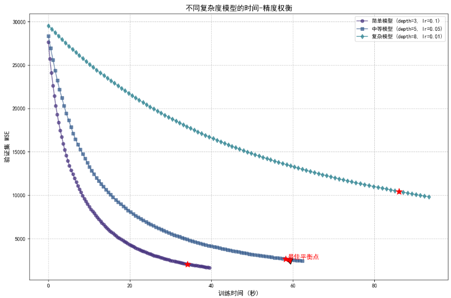
训练与验证损失对比
# 2. 训练与验证损失对比
import numpy as np
import matplotlib.pyplot as plt
from sklearn.datasets import make_regression
from sklearn.ensemble import GradientBoostingRegressor
from sklearn.model_selection import train_test_split
from sklearn.metrics import mean_squared_error
import time
import seaborn as sns# 设置样式
plt.rcParams['font.sans-serif'] = ['SimHei']
plt.rcParams['axes.unicode_minus'] = False
sns.set_palette("viridis")X, y = make_regression(n_samples=10000, n_features=50, noise=0.2, random_state=42)
X_train, X_test, y_train, y_test = train_test_split(X, y, test_size=0.2, random_state=42)# 模拟不同训练策略的结果
def simulate_training(model, max_iter=100):"""模拟训练过程并记录时间和精度"""train_losses = []val_losses = []times = []# 初始模型model.warm_start = Truemodel.n_estimators = 1model.fit(X_train, y_train)start_time = time.time()for i in range(1, max_iter + 1):model.n_estimators = imodel.fit(X_train, y_train)# 记录时间elapsed = time.time() - start_timetimes.append(elapsed)# 记录训练损失train_pred = model.predict(X_train)train_loss = mean_squared_error(y_train, train_pred)train_losses.append(train_loss)# 记录验证损失val_pred = model.predict(X_test)val_loss = mean_squared_error(y_test, val_pred)val_losses.append(val_loss)return np.array(times), np.array(train_losses), np.array(val_losses)model_simple = GradientBoostingRegressor(learning_rate=0.1, max_depth=3, random_state=42)
model_medium = GradientBoostingRegressor(learning_rate=0.05, max_depth=5, random_state=42)
model_complex = GradientBoostingRegressor(learning_rate=0.01, max_depth=8, random_state=42)# 模拟训练过程
times_simple, train_loss_simple, val_loss_simple = simulate_training(model_simple, 100)
times_medium, train_loss_medium, val_loss_medium = simulate_training(model_medium, 100)
times_complex, train_loss_complex, val_loss_complex = simulate_training(model_complex, 100)# 标记最佳平衡点(最大曲率点)
def find_elbow_point(times, losses):"""找到曲线的拐点(最大曲率点)"""# 计算一阶导数(梯度)grad = np.gradient(losses, times)# 计算二阶导数grad2 = np.gradient(grad, times)# 计算曲率curvature = np.abs(grad2) / (1 + grad ** 2) ** 1.5# 找到最大曲率点(排除前10%的点)exclude_n = max(5, int(len(curvature) * 0.1))max_idx = np.argmax(curvature[exclude_n:-5]) + exclude_nreturn times[max_idx], losses[max_idx]elbow_time_simple, elbow_loss_simple = find_elbow_point(times_simple, val_loss_simple)
elbow_time_medium, elbow_loss_medium = find_elbow_point(times_medium, val_loss_medium)
elbow_time_complex, elbow_loss_complex = find_elbow_point(times_complex, val_loss_complex)plt.figure(figsize=(12, 8))
plt.plot(times_medium, train_loss_medium, 'b-', label='训练损失')
plt.plot(times_medium, val_loss_medium, 'r-', label='验证损失')# 标记过拟合开始点
diff = val_loss_medium - train_loss_medium
overfit_idx = np.where(diff > np.percentile(diff, 90))[0][0]
overfit_time = times_medium[overfit_idx]
overfit_val_loss = val_loss_medium[overfit_idx]plt.axvline(x=overfit_time, color='purple', linestyle='--', alpha=0.7)
plt.scatter(overfit_time, overfit_val_loss, s=150, c='purple', marker='x')plt.annotate('过拟合开始点',(overfit_time, overfit_val_loss),xytext=(overfit_time+0.5, overfit_val_loss+5),arrowprops=dict(facecolor='purple', shrink=0.05, width=2),fontsize=12, color='purple')# 标记最佳点
plt.scatter(elbow_time_medium, elbow_loss_medium, s=150, c='red', marker='*', zorder=10)
plt.annotate('最佳平衡点',(elbow_time_medium, elbow_loss_medium),xytext=(elbow_time_medium+0.5, elbow_loss_medium+2),arrowprops=dict(facecolor='red', shrink=0.05, width=2),fontsize=12, color='red')plt.xlabel('训练时间 (秒)', fontsize=12)
plt.ylabel('MSE', fontsize=12)
plt.title('训练与验证损失随时间变化', fontsize=14)
plt.legend()
plt.grid(True, linestyle='--', alpha=0.7)
plt.tight_layout()
plt.show()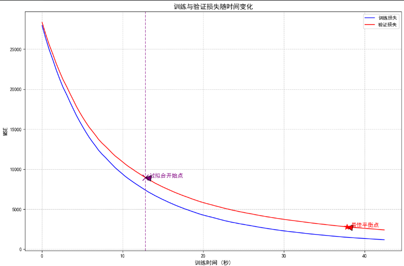
帕累托前沿分析(3D)
# 3. 帕累托前沿分析 (3D)
# 模拟不同超参数配置的结果import numpy as np
import matplotlib.pyplot as plt
from sklearn.datasets import make_regression
from sklearn.ensemble import GradientBoostingRegressor
from sklearn.model_selection import train_test_split
from sklearn.metrics import mean_squared_error
import time
import pandas as pd
import seaborn as sns# 设置样式
plt.rcParams['font.sans-serif'] = ['SimHei']
plt.rcParams['axes.unicode_minus'] = False
sns.set_palette("viridis")X, y = make_regression(n_samples=10000, n_features=50, noise=0.2, random_state=42)
X_train, X_test, y_train, y_test = train_test_split(X, y, test_size=0.2, random_state=42)
np.random.seed(42)
results = []
for _ in range(10):depth = np.random.randint(3, 10)lr = 10 ** np.random.uniform(-2, -0.5)n_estimators = np.random.randint(20, 200)model = GradientBoostingRegressor(max_depth=depth,learning_rate=lr,n_estimators=n_estimators,random_state=42)start_time = time.time()model.fit(X_train, y_train)train_time = time.time() - start_timey_pred = model.predict(X_test)mse = mean_squared_error(y_test, y_pred)results.append({'depth': depth,'lr': lr,'n_estimators': n_estimators,'time': train_time,'mse': mse,'cost_score': 0.7 * mse + 0.3 * np.log1p(train_time)  # 自定义成本函数})# 转换为DataFrame
df = pd.DataFrame(results)# 找到帕累托前沿点
def is_pareto_efficient(costs):"""找到帕累托最优解"""is_efficient = np.ones(costs.shape[0], dtype=bool)for i, c in enumerate(costs):if is_efficient[i]:# 所有成本都小于等于当前点的点is_efficient[is_efficient] = np.any(costs[is_efficient] < c, axis=1)is_efficient[i] = True  # 保持当前点return is_efficientcosts = df[['mse', 'time']].values
pareto_mask = is_pareto_efficient(costs)
pareto_points = df[pareto_mask]# 3D可视化
fig = plt.figure(figsize=(14, 10))
ax = fig.add_subplot(111, projection='3d')# 绘制所有点
scatter = ax.scatter(df['depth'],df['lr'],df['n_estimators'],c=df['cost_score'],cmap='viridis',s=50,alpha=0.7,label='所有配置'
)# 绘制帕累托前沿点
pareto_scatter = ax.scatter(pareto_points['depth'],pareto_points['lr'],pareto_points['n_estimators'],c='red',s=100,edgecolors='black',label='帕累托前沿'
)# 标记最佳性价比点
best_idx = df['cost_score'].idxmin()
best_point = df.loc[best_idx]
ax.scatter(best_point['depth'],best_point['lr'],best_point['n_estimators'],c='gold',s=200,edgecolors='black',marker='*',label='最佳性价比'
)ax.set_xlabel('树深度', fontsize=12)
ax.set_ylabel('学习率', fontsize=12)
ax.set_zlabel('树数量', fontsize=12)
ax.set_title('超参数空间的帕累托前沿分析', fontsize=14)
ax.legend()# 添加颜色条
cbar = fig.colorbar(scatter, pad=0.1)
cbar.set_label('成本分数 (MSE + 时间成本)', fontsize=12)plt.tight_layout()
plt.show()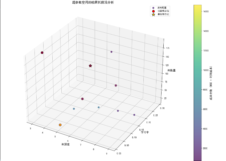


![[工具类] 网络请求HttpUtils](http://pic.xiahunao.cn/[工具类] 网络请求HttpUtils)
)
变换矩阵中的齐次坐标推导与几何理解)


)


——聚类算法KNN、Kmeans、Dbscan)
与另一个进程被死锁在锁资源上,并且已被选作死锁牺牲品。请重新运行该事务。不能在具有唯一索引“XXX_Index”的对象“dbo.Test”中插入重复键的行。)
