一、什么是 N-gram
核心定义:N-gram 是来自给定文本或语音序列的 N 个连续项(如单词、字符) 的序列。它是一种通过查看一个项目的前后文来建模序列的概率模型。
N: 代表连续项的数量。
项(Item): 通常是单词(Word),也可以是字符(Character)或音节。
核心思想:N-gram 模型基于一个简化的假设:一个词的出现概率只与它前面有限数量的词有关。这被称为马尔可夫假设。
例如,在一个 Trigram(3-gram)模型中,一个词的出现概率只由它前面的两个词决定,而不是整个句子的历史。这极大地简化了计算,使得处理大规模文本成为可能。
二、为什么需要 N-gram
在自然语言中,句子的概率是极其复杂的。要计算整个句子 P(“我今天学习N-gram”) 的联合概率,理论上需要知道所有词共同出现的概率,这在数据稀疏的现实世界中是不可能的。
N-gram 模型通过近似这个联合概率来解决这个问题。它将一个长序列的概率分解为一系列更短、更易计算的概率的乘积。
三、N-gram 的类型与示例
假设我们有一个句子:“我喜欢吃苹果”
Unigram (1-gram):
将文本视为独立的单词,不考虑任何上下文。
示例: [“我”], [“喜欢”], [“吃”], [“苹果”]
特点: 丢失了所有词序信息。
Bigram (2-gram):
每两个连续的单词作为一个单元。当前词的概率只依赖于前一个词。
示例: [“我”, “喜欢”], [“喜欢”, “吃”], [“吃”, “苹果”]
公式: P(句子) ≈ P(我) * P(喜欢|我) * P(吃|喜欢) * P(苹果|吃)
Trigram (3-gram):
每三个连续的单词作为一个单元。当前词的概率只依赖于前两个词。
示例: [“我”, “喜欢”, “吃”], [“喜欢”, “吃”, “苹果”]
公式: P(句子) ≈ P(我) * P(喜欢|我) * P(吃|我,喜欢) * P(苹果|喜欢,吃)
Four-gram (4-gram), Five-gram (5-gram)...
以此类推。N 越大,模型考虑的上下文就越长,理论上也越精确,但数据稀疏性问题也越严重。
示例:基于西雅图酒店数据集分析
import pandas as pd
from sklearn.metrics.pairwise import linear_kernel
from sklearn.feature_extraction.text import CountVectorizer
from sklearn.feature_extraction.text import TfidfVectorizer
import re
pd.options.display.max_columns = 30
import matplotlib.pyplot as plt
# 支持中文
plt.rcParams['font.sans-serif'] = ['SimHei'] # 用来正常显示中文标签
df = pd.read_csv('Seattle_Hotels.csv', encoding="latin-1")
# 数据探索
print(df.head())
print('数据集中的酒店个数:', len(df))
# 创建英文停用词列表
ENGLISH_STOPWORDS = {'i', 'me', 'my', 'myself', 'we', 'our', 'ours', 'ourselves', 'you', "you're", "you've", "you'll", "you'd", 'your', 'yours', 'yourself', 'yourselves', 'he', 'him', 'his', 'himself', 'she', "she's", 'her', 'hers', 'herself', 'it', "it's", 'its', 'itself', 'they', 'them', 'their', 'theirs', 'themselves', 'what', 'which', 'who', 'whom', 'this', 'that', "that'll", 'these', 'those', 'am', 'is', 'are', 'was', 'were', 'be', 'been', 'being', 'have', 'has', 'had', 'having', 'do', 'does', 'did', 'doing', 'a', 'an', 'the', 'and', 'but', 'if', 'or', 'because', 'as', 'until', 'while', 'of', 'at', 'by', 'for', 'with', 'about', 'against', 'between', 'into', 'through', 'during', 'before', 'after', 'above', 'below', 'to', 'from', 'up', 'down', 'in', 'out', 'on', 'off', 'over', 'under', 'again', 'further', 'then', 'once', 'here', 'there', 'when', 'where', 'why', 'how', 'all', 'any', 'both', 'each', 'few', 'more', 'most', 'other', 'some', 'such', 'no', 'nor', 'not', 'only', 'own', 'same', 'so', 'than', 'too', 'very', 's', 't', 'can', 'will', 'just', 'don', "don't", 'should', "should've", 'now', 'd', 'll', 'm', 'o', 're', 've', 'y', 'ain', 'aren', "aren't", 'couldn', "couldn't", 'didn', "didn't", 'doesn', "doesn't", 'hadn', "hadn't", 'hasn', "hasn't", 'haven', "haven't", 'isn', "isn't", 'ma', 'mightn', "mightn't", 'mustn', "mustn't", 'needn', "needn't", 'shan', "shan't", 'shouldn', "shouldn't", 'wasn', "wasn't", 'weren', "weren't", 'won', "won't", 'wouldn', "wouldn't"
}
def print_description(index):example = df[df.index == index][['desc', 'name']].values[0]if len(example) > 0:print(example[0])print('Name:', example[1])
print('第10个酒店的描述:')
print_description(10)
# 得到酒店描述中n-gram特征中的TopK个
def get_top_n_words(corpus, n=1, k=None):# 统计ngram词频矩阵,使用自定义停用词列表vec = CountVectorizer(ngram_range=(n, n), stop_words=list(ENGLISH_STOPWORDS)).fit(corpus)bag_of_words = vec.transform(corpus)"""print('feature names:')print(vec.get_feature_names())print('bag of words:')print(bag_of_words.toarray())"""sum_words = bag_of_words.sum(axis=0)words_freq = [(word, sum_words[0, idx]) for word, idx in vec.vocabulary_.items()]# 按照词频从大到小排序words_freq =sorted(words_freq, key = lambda x: x[1], reverse=True)return words_freq[:k]
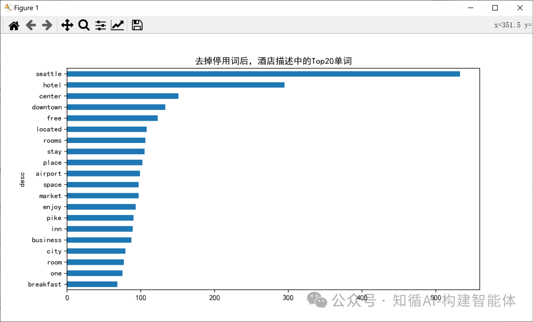
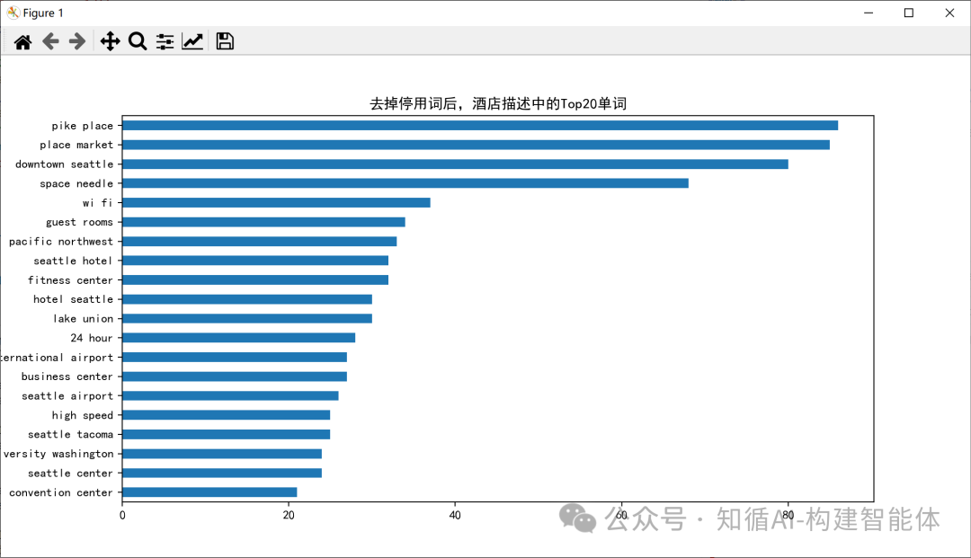
common_words = get_top_n_words(df['desc'], n=2, k=20)
#print(common_words)
df1 = pd.DataFrame(common_words, columns = ['desc' , 'count'])
df1.groupby('desc').sum()['count'].sort_values().plot(kind='barh', title='去掉停用词后,酒店描述中的Top20单词')
plt.show()
# 文本预处理
REPLACE_BY_SPACE_RE = re.compile('[/(){}\[\]\|@,;]')
BAD_SYMBOLS_RE = re.compile('[^0-9a-z #+_]')
# 使用自定义的英文停用词列表替代nltk的stopwords
STOPWORDS = ENGLISH_STOPWORDS
# 对文本进行清洗
def clean_text(text):# 全部小写text = text.lower()# 用空格替代一些特殊符号,如标点text = REPLACE_BY_SPACE_RE.sub(' ', text)# 移除BAD_SYMBOLS_REtext = BAD_SYMBOLS_RE.sub('', text)# 从文本中去掉停用词text = ' '.join(word for word in text.split() if word not in STOPWORDS) return text
# 对desc字段进行清理,apply针对某列
df['desc_clean'] = df['desc'].apply(clean_text)
#print(df['desc_clean'])
# 建模
df.set_index('name', inplace = True)
# 使用TF-IDF提取文本特征,使用自定义停用词列表
tf = TfidfVectorizer(analyzer='word', ngram_range=(1, 3), min_df=0.01, stop_words=list(ENGLISH_STOPWORDS))
# 针对desc_clean提取tfidf
tfidf_matrix = tf.fit_transform(df['desc_clean'])
print('TFIDF feature names:')
#print(tf.get_feature_names_out())
print(len(tf.get_feature_names_out()))
#print('tfidf_matrix:')
print(tfidf_matrix.shape)
# 计算酒店之间的余弦相似度(线性核函数)
cosine_similarities = linear_kernel(tfidf_matrix, tfidf_matrix)
#print(cosine_similarities)
print(cosine_similarities.shape)
indices = pd.Series(df.index) #df.index是酒店名称
# 基于相似度矩阵和指定的酒店name,推荐TOP10酒店
def recommendations(name, cosine_similarities = cosine_similarities):recommended_hotels = []# 找到想要查询酒店名称的idxidx = indices[indices == name].index[0]print('idx=', idx)# 对于idx酒店的余弦相似度向量按照从大到小进行排序score_series = pd.Series(cosine_similarities[idx]).sort_values(ascending = False)# 取相似度最大的前10个(除了自己以外)top_10_indexes = list(score_series.iloc[1:11].index)# 放到推荐列表中for i in top_10_indexes:recommended_hotels.append(list(df.index)[i])return recommended_hotels
print(recommendations('Hilton Seattle Airport & Conference Center'))
print(recommendations('The Bacon Mansion Bed and Breakfast'))
#print(result)Unigram (1-gram)结果:
Bigram (2-gram)结果:
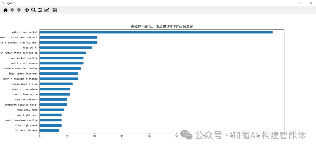
Trigram (3-gram)结果:
四、N-gram 的概率计算
N-gram 模型的核心是计算条件概率。我们通过在大型语料库中计数来估计这些概率。
最大似然估计(MLE)公式
对于 Bigram:
P(w_i | w_{i-1}) = Count(w_{i-1}, w_i) / Count(w_{i-1})
Count(w_{i-1}, w_i) 是序列 (w_{i-1}, w_i) 在语料库中出现的次数。
Count(w_{i-1}) 是单词 w_{i-1} 在语料库中出现的总次数。
具体示例:
假设我们的语料库由以下三个句子组成(<s> 和 </s> 是句首和句尾标记):
<s> 我喜欢吃苹果 </s>
<s> 我喜欢读书 </s>
<s> 你喜欢什么 </s>
现在,我们来计算一些概率:
P(喜欢 | 我) = Count(我, 喜欢) / Count(我)
Count(我, 喜欢) = 2 (在句子1和2中,“我喜欢”都出现了)
Count(我) = 2 (“我”作为第一个词出现了2次)
所以,P(喜欢 | 我) = 2 / 2 = 1.0
P(吃 | 喜欢) = Count(喜欢, 吃) / Count(喜欢)
Count(喜欢, 吃) = 1 (只在句子1中出现)
Count(喜欢) = 3 (在三个句子中都出现了“喜欢”)
所以,P(吃 | 喜欢) = 1 / 3 ≈ 0.33
P(苹果 | 吃) = Count(吃, 苹果) / Count(吃)
Count(吃, 苹果) = 1
Count(吃) = 1
所以,P(苹果 | 吃) = 1 / 1 = 1.0
现在,计算整个句子 “我喜欢吃苹果” 的 Bigram 概率:
P(句子) = P(我 | <s>) * P(喜欢 | 我) * P(吃 | 喜欢) * P(苹果 | 吃) * P(</s> | 苹果)
我们需要额外计算:
P(我 | <s>) = Count(<s>, 我) / Count(<s>) = 2 / 3(3个句子,2个以“我”开头)
P(</s> | 苹果) = Count(苹果, </s>) / Count(苹果) = 1 / 1 = 1.0(假设“苹果”只在句尾出现一次)
最终:
P(句子) = (2/3) * 1.0 * (1/3) * 1.0 * 1.0 ≈ 0.222
马尔可夫假设
N-Gram基于一个巧妙而有效的简化:一个词的出现概率只与它前面有限个词有关。这一假设使得复杂的语言建模问题变得可计算。例如,在Bigram模型中,我们假设:P(天气|今天) ≈ P(天气|今天)
N-Gram模型的核心是计算序列概率。对于一个句子"今天天气真好",其概率可以表示为:
P(今天天气真好) = P(今天) × P(天气|今天) × P(真|天气) × P(好|真)
假设语料库中有以下句子:
今天天气真好
今天心情真好
明天天气不错
计算P(天气|今天):
Count(今天, 天气) = 1(第1句)
Count(今天) = 2(第1、2句)
P(天气|今天) = 1/2 = 0.5
参考代码:
from collections import defaultdict, Counter
import numpy as np
# 简单语料库
corpus = [['今天', '天气', '真好'],['今天', '心情', '真好'], ['明天', '天气', '不错']
]
# 构建Bigram模型
def build_bigram_model(corpus):bigram_counts = defaultdict(Counter)unigram_counts = Counter()for sentence in corpus:for i in range(len(sentence)-1):current_word = sentence[i]next_word = sentence[i+1]bigram_counts[current_word][next_word] += 1unigram_counts[current_word] += 1# 计算概率bigram_probs = {}for prev_word, next_words in bigram_counts.items():total = unigram_counts[prev_word]bigram_probs[prev_word] = {next_word: count/total for next_word, count in next_words.items()}return bigram_probs
# 构建模型
model = build_bigram_model(corpus)
print("P(天气|今天) =", model['今天']['天气'])
print("P(心情|今天) =", model['今天']['心情'])
输出结果:
P(天气|今天) = 0.5
P(心情|今天) = 0.5基于以上基础继续实现文本自动生成:
def generate_text(seed_word, model, length=10):current_word = seed_wordgenerated_text = [current_word]for _ in range(length-1):if current_word not in model:breaknext_words = list(model[current_word].keys())probabilities = list(model[current_word].values())# 按概率选择下一个词next_word = np.random.choice(next_words, p=probabilities)generated_text.append(next_word)current_word = next_wordreturn ''.join(generated_text)
# 生成文本
print("生成示例:", generate_text('今天', model, 5))
输出结果:
生成示例: 今天天气真好参考经典的硬币投掷问题加深理解:
最大似然估计(MLE)是统计学中一种常用的参数估计方法。它的核心思想是:在已知数据集的情况下,寻找最有可能产生这些数据的参数值。
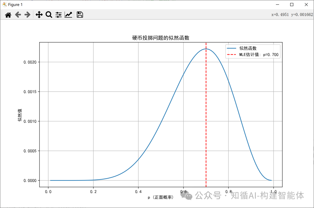
举个例子,假设我们有一个硬币,我们想估计掷硬币时正面朝上的概率p。我们掷了10次硬币,结果有7次正面朝上,3次反面朝上。我们可以将每次掷硬币看作是一个伯努利试验,那么正面朝上的次数X服从二项分布,即X ~ Binomial(n=10, p)。
我们的目标是估计参数p。似然函数就是给定参数p时,观察到当前数据的概率。对于二项分布,似然函数为:
L(p) = P(X=7 | p) = C(10,7) * p^7 * (1-p)^3
最大似然估计就是要找到使L(p)最大的p值。通常,我们会取似然函数的对数(因为对数函数是单调的,最大化对数似然等价于最大化似然),然后求导并令导数为0。
对数似然函数为:log L(p) = log(C(10,7)) + 7*log(p) + 3*log(1-p)
对p求导并令导数为0:d(log L(p))/dp = 7/p - 3/(1-p) = 0
解方程:7/p = 3/(1-p) => 7(1-p) = 3p => 7 - 7p = 3p => 7 = 10p => p = 0.7
因此,p的最大似然估计值是0.7。
下面我们用Python代码来演示这个过程,包括绘制似然函数曲线。
mport numpy as np
import matplotlib.pyplot as plt
from scipy.optimize import minimize_scalar
# 设置matplotlib支持中文显示
plt.rcParams['font.sans-serif'] = ['SimHei']  # 用来正常显示中文标签
plt.rcParams['axes.unicode_minus'] = False  # 用来正常显示负号
# 观测数据:7次正面,3次反面
data = np.array([1, 1, 1, 1, 1, 1, 1, 0, 0, 0])
n_heads = np.sum(data)
n_tails = len(data) - n_heads
# 定义似然函数
def likelihood(p):return p**n_heads * (1-p)**n_tails
# 定义负对数似然函数(因为我们要最小化)
def neg_log_likelihood(p):return - (n_heads * np.log(p) + n_tails * np.log(1-p))
# 使用优化方法找到最大似然估计
result = minimize_scalar(neg_log_likelihood, bounds=(0.01, 0.99), method='bounded')
mle_p = result.x
print(f"最大似然估计值: p = {mle_p:.3f}")
# 可视化似然函数
p_values = np.linspace(0.01, 0.99, 100)
likelihood_values = [likelihood(p) for p in p_values]
plt.figure(figsize=(10, 6))
plt.plot(p_values, likelihood_values, label='似然函数')
plt.axvline(mle_p, color='r', linestyle='--', label=f'MLE估计值: p={mle_p:.3f}')
plt.xlabel('p (正面概率)')
plt.ylabel('似然值')
plt.title('硬币投掷问题的似然函数')
plt.legend()
plt.grid(True)
plt.show()
结果展示:
五、数据稀疏与平滑技术
如果语料库中从未出现过 (w_{i-1}, w_i) 这个组合,那么 P(w_i | w_{i-1}) = 0,这会导致整个句子的概率为0。例如,语料库中如果没有“吃香蕉”,那么句子“我喜欢吃香蕉”的概率就是0,这显然不合理。
解决方案: 平滑(Smoothing)技术。其核心思想是从已知概率中“偷”一点概率质量分配给未出现过的序列。
常见平滑方法:
加一平滑(Add-One / Laplace Smoothing): 将所有计数加1,避免0概率。
古德-图灵估计(Good-Turing Estimation): 用出现一次的事物的数量来估计未出现事物的概率。
回退(Backoff): 如果N-gram不存在,就回退到使用 (N-1)-gram 的概率。
插值(Interpolation): 将不同阶数的N-gram(如unigram, bigram, trigram)的概率加权混合起来。
六、N-gram 的应用
文本生成:
给定一个起始词,根据N-gram概率选择下一个最可能的词,依此类推,生成连贯的文本。
示例: 输入“今天”,模型可能根据语料库生成“今天天气真好”。
语法检查与纠错:
低概率的单词序列很可能存在语法错误或拼写错误。
示例: “吃飞机”这个Bigram的概率极低,系统会提示“吃飞机”可能应为“坐飞机”。
输入法预测:
当你输入“wo”时,输入法会预测“我”;当你输入“wo xihuan”时,它会预测“我喜欢”以及后续可能接的词“读书”、“吃”等。
语音识别:
帮助系统在发音相近的候选词中选择最符合上下文语境的词。
示例: 识别到发音为“shi4 jian4”,在“事件”和“时间”之间,如果上文是“漫长的”,则选择“时间”的概率更高。
机器翻译:
用于评估翻译输出的流畅度,选择那些听起来更自然、更符合目标语言N-gram习惯的译文。
信息检索:
处理短语查询(如“纽约时报”),将其视为一个Bigram,比单独搜索“纽约”和“时报”能返回更精确的结果。
七、总结
N-gram 是一个简单而强大的概率模型,用于表示文本中的连续序列。通过有限的上下文来捕捉语言的局部规律,平衡了模型的复杂度和计算可行性。虽然如今Transformer(如BERT, GPT)等深度学习模型在大多数NLP任务上超越了N-gram,但N-gram因其轻量、可解释、不需要训练(仅需计数)的特性,在资源受限的场景、快速原型开发以及作为大型模型的补充组件中,依然发挥着重要作用。理解N-gram是理解更复杂NLP模型的基础。
)


精讲)


:构建企业知识库,深入ETL与RAG实现)


)


基本控件应用)


