[深度学习]目标检测基础

一、实验目的

二、实验环境

三、实验内容

3.1 LM_BoundBox

3.1.1 实验代码

3.1.2 实验结果

3.2 LM_Anchor

3.2.1 实验代码

3.2.2 实验结果

3.3 LM_Multiscale-object-detection

3.3.1 实验代码

3.3.2 实验结果

四、实验小结

一、实验目的

了解python语法
了解目标检测的原理
了解边界框、锚框、多尺度目标检测的实现

二、实验环境

Baidu 飞桨AI Studio

三、实验内容

3.1 LM_BoundBox

3.1.1 实验代码

%matplotlib inline
import torch
from d2l import torch as d2l
d2l.set_figsize()
img = d2l.plt.imread('./img/catdog.jpg')
d2l.plt.imshow(img);def box_corner_to_center(boxes):x1, y1, x2, y2 = boxes[:, 0], boxes[:, 1], boxes[:, 2], boxes[:, 3]cx = (x1 + x2) / 2cy = (y1 + y2) / 2w = x2 - x1h = y2 - y1boxes = torch.stack((cx, cy, w, h), axis=-1)return boxesdef box_center_to_corner(boxes):cx, cy, w, h = boxes[:, 0], boxes[:, 1], boxes[:, 2], boxes[:, 3]x1 = cx - 0.5 * wy1 = cy - 0.5 * hx2 = cx + 0.5 * wy2 = cy + 0.5 * hboxes = torch.stack((x1, y1, x2, y2), axis=-1)return boxes
dog_bbox , cat_bbox=[60.0, 45.0, 378.0, 516.0], [400.0, 112.0, 655.0, 493.0] 
boxes = torch.tensor((dog_bbox, cat_bbox))
box_center_to_corner(box_corner_to_center(boxes)) == boxesdef bbox_to_rect(bbox, color):return d2l.plt.Rectangle(xy=(bbox[0], bbox[1]), width=bbox[2]-bbox[0], height=bbox[3]-bbox[1],fill=False, edgecolor=color, linewidth=2)
fig = d2l.plt.imshow(img)
fig.axes.add_patch(bbox_to_rect(dog_bbox, 'blue'))
fig.axes.add_patch(bbox_to_rect(cat_bbox, 'red'));

import torch
from d2l import torch as d2l
d2l.set_figsize()
img2=d2l.plt.imread('./img/dog1.jpg')
d2l.plt.imshow(img2);
def box_corner_to_center(boxes):x1, y1, x2, y2 = boxes[:, 0], boxes[:, 1], boxes[:, 2], boxes[:, 3]cx = (x1 + x2) / 2cy = (y1 + y2) / 2w = x2 - x1h = y2 - y1boxes = torch.stack((cx, cy, w, h), axis=-1)return boxes
def box_center_to_corner(boxes):cx, cy, w, h = boxes[:, 0], boxes[:, 1], boxes[:, 2], boxes[:, 3]x1 = cx - 0.5 * wy1 = cy - 0.5 * hx2 = cx + 0.5 * wy2 = cy + 0.5 * hboxes = torch.stack((x1, y1, x2, y2), axis=-1)
return boxes
dog_box=[250.0,50.0,1080.0,1200.0]
box_test = torch.tensor(dog_box).view(1, -1)
centered_box = box_corner_to_center(box_test)
print("Centered box:", centered_box)cornered_box = box_center_to_corner(centered_box)
print("Cornered box:", cornered_box)
def bbox_to_rect(bbox, color):return d2l.plt.Rectangle(xy=(bbox[0], bbox[1]), width=bbox[2]-bbox[0], height=bbox[3]-bbox[1],fill=False, edgecolor=color, linewidth=2)
fig = d2l.plt.imshow(img2)
fig.axes.add_patch(bbox_to_rect(dog_box, 'blue'))

代码分析：

在代码中，定义两种对边界框的表示，box_corner_to_center从两角表示转换为中心宽度表示，而box_center_to_corner从中心宽度表示转换为两角表示。输入参数boxes可以是长度为4的张量，也可以是形状为（nn，4）的二维张量，其中nn是边界框的数量。将边界框在图中画出，定义一个辅助函数bbox_to_rect。它将边界框表示成matplotlib的边界框格式。

3.1.2 实验结果

如下图所示，在下面图像中标记图像中包含对象的边界框。

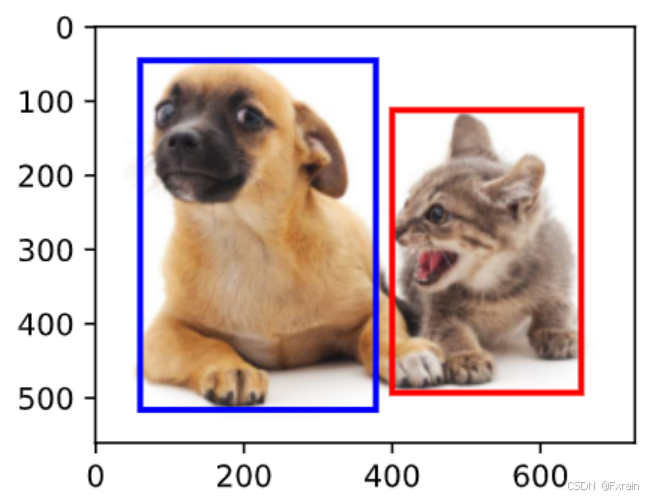
图 1

常见的边界框表示方法有两种：

1.角点表示法：用左上角和右下角的坐标来表示边界框。例如，对于边界框 (x1, y1, x2, y2)，其中 (x1, y1) 是左上角的坐标，(x2, y2) 是右下角的坐标。

2.中心点表示法：用中心点的坐标、宽度和高度来表示边界框。例如，对于边界框 (cx, cy, w, h)，其中 (cx, cy) 是中心点的坐标，w 是宽度，h 是高度。函数 box_corner_to_center 和 box_center_to_corner 分别实现了从角点表示法到中心点表示法的转换，以及从中心点表示法到角点表示法的转换。

在这两个函数中，输入参数的最内层维度总是4，这是因为每个边界框需要四个值来表示其位置信息。无论是使用角点表示法还是中心点表示法，都需要这四个值：对于角点表示法，需要 (x1, y1, x2, y2) 四个值。对于中心点表示法，需要 (cx, cy, w, h) 四个值。因此，输入参数的最内层维度总是4。

3.2 LM_Anchor

3.2.1 实验代码

%matplotlib inline
import torch
from d2l import torch as d2ltorch.set_printoptions(2)  def multibox_prior(data, sizes, ratios):in_height, in_width = data.shape[-2:]device, num_sizes, num_ratios = data.device, len(sizes), len(ratios)boxes_per_pixel = (num_sizes + num_ratios - 1)size_tensor = torch.tensor(sizes, device=device)ratio_tensor = torch.tensor(ratios, device=device)offset_h, offset_w = 0.5, 0.5steps_h = 1.0 / in_height  steps_w = 1.0 / in_width center_h = (torch.arange(in_height, device=device) + offset_h) * steps_hcenter_w = (torch.arange(in_width, device=device) + offset_w) * steps_wshift_y, shift_x = torch.meshgrid(center_h, center_w)shift_y, shift_x = shift_y.reshape(-1), shift_x.reshape(-1)w = torch.cat((size_tensor * torch.sqrt(ratio_tensor[0]),sizes[0] * torch.sqrt(ratio_tensor[1:])))\* in_height / in_width  h = torch.cat((size_tensor / torch.sqrt(ratio_tensor[0]),sizes[0] / torch.sqrt(ratio_tensor[1:])))anchor_manipulations = torch.stack((-w, -h, w, h)).T.repeat(in_height * in_width, 1) / 2out_grid = torch.stack([shift_x, shift_y, shift_x, shift_y],dim=1).repeat_interleave(boxes_per_pixel, dim=0)output = out_grid + anchor_manipulationsreturn output.unsqueeze(0)img = d2l.plt.imread('./img/catdog.jpg')
h, w = img.shape[:2]print(h, w)
X = torch.rand(size=(1, 3, h, w))
Y = multibox_prior(X, sizes=[0.75, 0.5, 0.25], ratios=[1, 2, 0.5])
Y.shapeboxes = Y.reshape(h, w, 5, 4)
boxes[250, 250, 0, :]def show_bboxes(axes, bboxes, labels=None, colors=None):def _make_list(obj, default_values=None):if obj is None:obj = default_valueselif not isinstance(obj, (list, tuple)):obj = [obj]return objlabels = _make_list(labels)colors = _make_list(colors, ['b', 'g', 'r', 'm', 'c'])for i, bbox in enumerate(bboxes):color = colors[i % len(colors)]rect = d2l.bbox_to_rect(bbox.detach().numpy(), color)axes.add_patch(rect)if labels and len(labels) > i:text_color = 'k' if color == 'w' else 'w'axes.text(rect.xy[0], rect.xy[1], labels[i],va='center', ha='center', fontsize=9, color=text_color,bbox=dict(facecolor=color, lw=0))d2l.set_figsize()
bbox_scale = torch.tensor((w, h, w, h))
fig = d2l.plt.imshow(img)
show_bboxes(fig.axes, boxes[250, 250, :, :] * bbox_scale,['s=0.75, r=1', 's=0.5, r=1', 's=0.25, r=1', 's=0.75, r=2','s=0.75, r=0.5'])def box_iou(boxes1, boxes2):box_area = lambda boxes: ((boxes[:, 2] - boxes[:, 0]) *(boxes[:, 3] - boxes[:, 1]))areas1 = box_area(boxes1)areas2 = box_area(boxes2)inter_upperlefts = torch.max(boxes1[:, None, :2], boxes2[:, :2])inter_lowerrights = torch.min(boxes1[:, None, 2:], boxes2[:, 2:])inters = (inter_lowerrights - inter_upperlefts).clamp(min=0)inter_areas = inters[:, :, 0] * inters[:, :, 1]union_areas = areas1[:, None] + areas2 - inter_areasreturn inter_areas / union_areasdef assign_anchor_to_bbox(ground_truth, anchors, device, iou_threshold=0.5):num_anchors, num_gt_boxes = anchors.shape[0], ground_truth.shape[0]jaccard = box_iou(anchors, ground_truth)anchors_bbox_map = torch.full((num_anchors,), -1, dtype=torch.long,device=device)max_ious, indices = torch.max(jaccard, dim=1)anc_i = torch.nonzero(max_ious >= 0.5).reshape(-1)box_j = indices[max_ious >= 0.5]anchors_bbox_map[anc_i] = box_jcol_discard = torch.full((num_anchors,), -1)row_discard = torch.full((num_gt_boxes,), -1)for _ in range(num_gt_boxes):max_idx = torch.argmax(jaccard)box_idx = (max_idx % num_gt_boxes).long()anc_idx = (max_idx / num_gt_boxes).long()anchors_bbox_map[anc_idx] = box_idxjaccard[:, box_idx] = col_discardjaccard[anc_idx, :] = row_discardreturn anchors_bbox_mapdef offset_boxes(anchors, assigned_bb, eps=1e-6):c_anc = d2l.box_corner_to_center(anchors)c_assigned_bb = d2l.box_corner_to_center(assigned_bb)offset_xy = 10 * (c_assigned_bb[:, :2] - c_anc[:, :2]) / c_anc[:, 2:]offset_wh = 5 * torch.log(eps + c_assigned_bb[:, 2:] / c_anc[:, 2:])offset = torch.cat([offset_xy, offset_wh], axis=1)return offsetdef multibox_target(anchors, labels):batch_size, anchors = labels.shape[0], anchors.squeeze(0)batch_offset, batch_mask, batch_class_labels = [], [], []device, num_anchors = anchors.device, anchors.shape[0]for i in range(batch_size):label = labels[i, :, :]anchors_bbox_map = assign_anchor_to_bbox(label[:, 1:], anchors, device)bbox_mask = ((anchors_bbox_map >= 0).float().unsqueeze(-1)).repeat(1, 4)class_labels = torch.zeros(num_anchors, dtype=torch.long,device=device)assigned_bb = torch.zeros((num_anchors, 4), dtype=torch.float32,device=device)indices_true = torch.nonzero(anchors_bbox_map >= 0)bb_idx = anchors_bbox_map[indices_true]class_labels[indices_true] = label[bb_idx, 0].long() + 1assigned_bb[indices_true] = label[bb_idx, 1:]offset = offset_boxes(anchors, assigned_bb) * bbox_maskbatch_offset.append(offset.reshape(-1))batch_mask.append(bbox_mask.reshape(-1))batch_class_labels.append(class_labels)bbox_offset = torch.stack(batch_offset)bbox_mask = torch.stack(batch_mask)class_labels = torch.stack(batch_class_labels)return (bbox_offset, bbox_mask, class_labels)ground_truth = torch.tensor([[0, 0.1, 0.08, 0.52, 0.92],[1, 0.55, 0.2, 0.9, 0.88]])
anchors = torch.tensor([[0, 0.1, 0.2, 0.3], [0.15, 0.2, 0.4, 0.4],[0.63, 0.05, 0.88, 0.98], [0.66, 0.45, 0.8, 0.8],[0.57, 0.3, 0.92, 0.9]])fig = d2l.plt.imshow(img)
show_bboxes(fig.axes, ground_truth[:, 1:] * bbox_scale, ['dog', 'cat'], 'k')
show_bboxes(fig.axes, anchors * bbox_scale, ['0', '1', '2', '3', '4']);labels = multibox_target(anchors.unsqueeze(dim=0),ground_truth.unsqueeze(dim=0))
def offset_inverse(anchors, offset_preds):anc = d2l.box_corner_to_center(anchors)pred_bbox_xy = (offset_preds[:, :2] * anc[:, 2:] / 10) + anc[:, :2]pred_bbox_wh = torch.exp(offset_preds[:, 2:] / 5) * anc[:, 2:]pred_bbox = torch.cat((pred_bbox_xy, pred_bbox_wh), axis=1)predicted_bbox = d2l.box_center_to_corner(pred_bbox)return predicted_bbox
def nms(boxes, scores, iou_threshold):B = torch.argsort(scores, dim=-1, descending=True)keep = [] while B.numel() > 0:i = B[0]keep.append(i)if B.numel() == 1: breakiou = box_iou(boxes[i, :].reshape(-1, 4),boxes[B[1:], :].reshape(-1, 4)).reshape(-1)inds = torch.nonzero(iou <= iou_threshold).reshape(-1)B = B[inds + 1]return torch.tensor(keep, device=boxes.device)def multibox_detection(cls_probs, offset_preds, anchors, nms_threshold=0.5,pos_threshold=0.009999999):device, batch_size = cls_probs.device, cls_probs.shape[0]anchors = anchors.squeeze(0)num_classes, num_anchors = cls_probs.shape[1], cls_probs.shape[2]out = []for i in range(batch_size):cls_prob, offset_pred = cls_probs[i], offset_preds[i].reshape(-1, 4)conf, class_id = torch.max(cls_prob[1:], 0)predicted_bb = offset_inverse(anchors, offset_pred)keep = nms(predicted_bb, conf, nms_threshold)all_idx = torch.arange(num_anchors, dtype=torch.long, device=device)combined = torch.cat((keep, all_idx))uniques, counts = combined.unique(return_counts=True)non_keep = uniques[counts == 1]all_id_sorted = torch.cat((keep, non_keep))class_id[non_keep] = -1class_id = class_id[all_id_sorted]conf, predicted_bb = conf[all_id_sorted], predicted_bb[all_id_sorted]below_min_idx = (conf < pos_threshold)class_id[below_min_idx] = -1conf[below_min_idx] = 1 - conf[below_min_idx]pred_info = torch.cat((class_id.unsqueeze(1),conf.unsqueeze(1),predicted_bb), dim=1)out.append(pred_info)return torch.stack(out)
anchors = torch.tensor([[0.1, 0.08, 0.52, 0.92], [0.08, 0.2, 0.56, 0.95],[0.15, 0.3, 0.62, 0.91], [0.55, 0.2, 0.9, 0.88]])
offset_preds = torch.tensor([0] * anchors.numel())
cls_probs = torch.tensor([[0] * 4, [0.9, 0.8, 0.7, 0.1], [0.1, 0.2, 0.3, 0.9]]) 
fig = d2l.plt.imshow(img)
show_bboxes(fig.axes, anchors * bbox_scale,['dog=0.9', 'dog=0.8', 'dog=0.7', 'cat=0.9'])
output = multibox_detection(cls_probs.unsqueeze(dim=0),offset_preds.unsqueeze(dim=0),anchors.unsqueeze(dim=0),nms_threshold=0.5)
output
fig = d2l.plt.imshow(img)
for i in output[0].detach().numpy():if i[0] == -1:continuelabel = ('dog=', 'cat=')[int(i[0])] + str(i[1])show_bboxes(fig.axes, [torch.tensor(i[2:]) * bbox_scale], label)

代码分析：

假设输入图像的高度为hh，宽度为ww。我们以图像的每个像素为中心生成不同形状的锚框：比例为s∈(0,1]s∈(0,1]，宽高比（宽高比）为r>0r>0。multibox_prior函数实现生成锚框，指定输入图像、尺度列表和宽高比列表，然后此函数将返回所有的锚框。将锚框变量Y的形状更改为（图像高度、图像宽度、以同一像素为中心的锚框的数量，4）后，可以获得以指定像素的位置为中心的所有锚框。 [访问以（250,250）为中心的第一个锚框]，它有四个元素：锚框左上角的(x,y)(x,y)轴坐标和右下角的(x,y)(x,y)轴坐标。将两个轴的坐标分别除以图像的宽度和高度后，所得的值就介于0和1之间。定义show_bboxes函数来在图像上绘制多个边界框。

计算交并比来衡量锚框和真实边界框之间、以及不同锚框之间的相似度。给定两个锚框或边界框的列表，通过box_iou函数在这两个列表中计算它们成对的交并比。将真实边界框分配给锚框，为每个锚框标记类别和偏移量。通过offset_inverse函数将锚框和偏移量预测作为输入，并[应用逆偏移变换来返回预测的边界框坐标]。再使用非极大值抑制（non-maximum suppression，NMS）合并属于同一目标的类似的预测边界框。最后返回预测边界框和置信度。

3.2.2 实验结果

（1）如下图所示，在图像中绘制锚框，并标记锚框的高宽比和缩放比

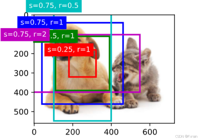
图 3

(2)如下图所示，在图像中绘制边界框和锚框，边界框返回目标的类别（这里为“dog”和“cat”）。

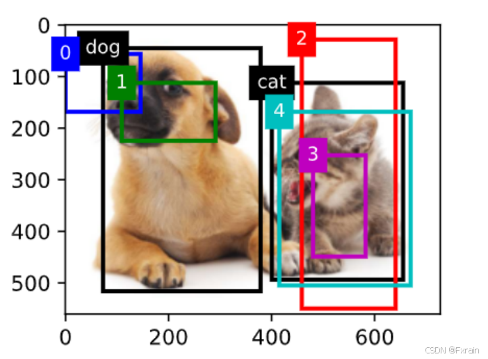
图 4

(3)如下图所示，在图像上绘制预测边界框和置信度

图 6

(4)如下图所示，输出由非极大值抑制保存的最终预测边界框

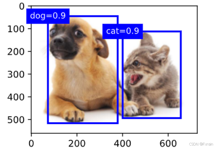
图 7

在 multibox_prior 函数中，sizes 和 ratios 参数决定了生成的锚框的大小和长宽比。这些参数的变化将直接影响生成的锚框的形状和分布。

（1）改变 sizes 参数。如果增加了 sizes 中的值，那么生成的锚框将会更大。如果减少了 sizes 中的值，那么生成的锚框将会更小。

（2）改变 ratios 参数。如果增加了 ratios 中的值，那么生成的锚框将会有更多不同的长宽比。如果减少了 ratios 中的值，那么生成的锚框将会更少地覆盖不同的长宽比。

如果需要构建并可视化两个IoU为0.5的边界框，则代码如下：

import torchimport matplotlib.pyplot as pltimport matplotlib.patches as patchesdef box_iou(boxes1, boxes2):area1 = (boxes1[:, 2] - boxes1[:, 0]) * (boxes1[:, 3] - boxes1[:, 1])area2 = (boxes2[:, 2] - boxes2[:, 0]) * (boxes2[:, 3] - boxes2[:, 1])lt = torch.max(boxes1[:, None, :2], boxes2[:, :2]) rb = torch.min(boxes1[:, None, 2:], boxes2[:, 2:])  wh = (rb - lt).clamp(min=0)  inter = wh[:, :, 0] * wh[:, :, 1]  union = area1[:, None] + area2 - inter  return inter / uniondef visualize_iou_boxes(image, ground_truth, anchors, iou_threshold=0.5):jaccard = box_iou(anchors, ground_truth)max_ious, indices = torch.max(jaccard, dim=1)anc_i = torch.nonzero(max_ious >= iou_threshold).reshape(-1)box_j = indices[max_ious >= iou_threshold]fig, ax = plt.subplots(1)ax.imshow(image)for i in range(len(anc_i)):anchor = anchors[anc_i[i]]gt_box = ground_truth[box_j[i]]rect = patches.Rectangle((anchor[0], anchor[1]), anchor[2] - anchor[0], anchor[3] - anchor[1],linewidth=1, edgecolor='k', facecolor='none')ax.add_patch(rect)rect = patches.Rectangle((gt_box[0], gt_box[1]), gt_box[2] - gt_box[0], gt_box[3] - gt_box[1],linewidth=1, edgecolor='b', facecolor='none')ax.add_patch(rect)plt.show()image = plt.imread('./img/catdog.jpg') ground_truth = torch.tensor([[50, 50, 400, 480], [420, 150, 650, 480]])  anchors = torch.tensor([[60, 60, 380, 420], [420, 190, 600, 450], [100, 100, 200, 200],[450,200,600,350]])  visualize_iou_boxes(image, ground_truth, anchors, iou_threshold=0.5)

结果如下图图10所示，其中蓝色为边界框，黑色为锚框。可以看到，

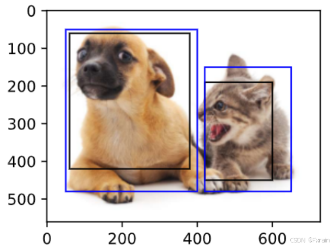
图 10

在:numref:subsec_labeling-anchor-boxes中修改anchors变量会导致重新计算所有锚框与真实边界框之间的 IoU，需要计算出新的IoU值。锚框的中心坐标和尺寸、中心坐标的偏移量、锚框的高宽比、最终的偏移量张量也会发生变化。总结来说，修改 anchors 会直接影响到锚框与真实边界框之间的映射关系、偏移量计算以及最终的掩码和类别标签，从而导致整个函数的输出结果发生变化。如图11所示，修改anchors后的锚框尺寸改变。

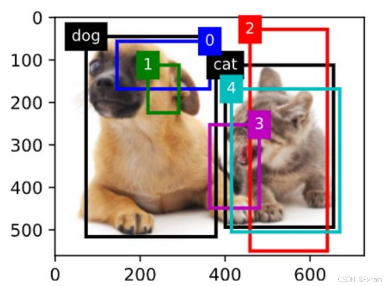
图 11

在:numref:subsec_predicting-bounding-boxes-nms中修改anchors变量会导致锚框的位置变化，新的 anchors 会影响生成的边界框的中心位置。如果 anchors 的中心位置不同，那么生成的边界框的中心也会相应地移动。由于边界框的位置和大小都发生了变化，最终的检测结果可能会有所不同。这可能会导致一些目标被正确检测到，而另一些目标则可能被漏检或误检。如图12、13、14所示，修改anchors后的锚框尺寸改变。

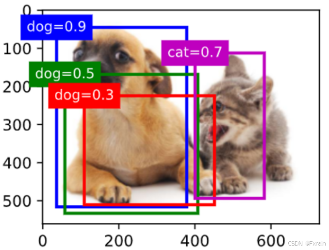
图 12

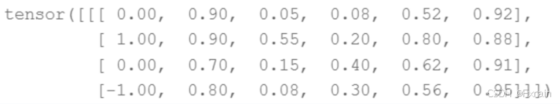
图 13

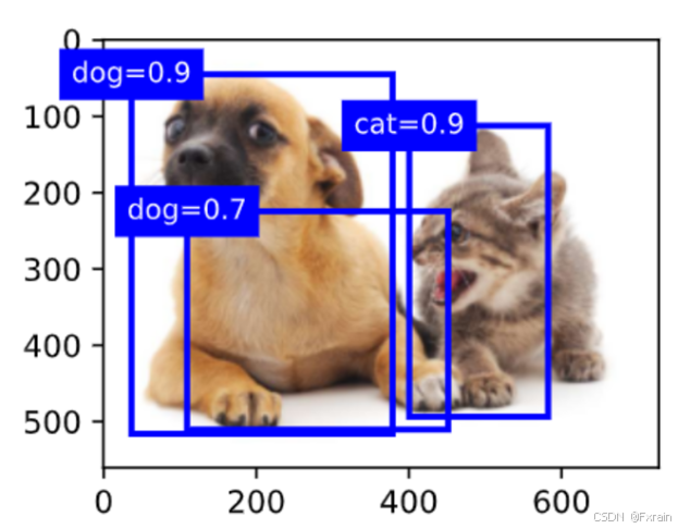
图 14

3.3 LM_Multiscale-object-detection

3.3.1 实验代码

%matplotlib inline
import torch
from d2l import torch as d2limg = d2l.plt.imread('./img/catdog.jpg')
h, w = img.shape[:2]
h, w
def display_anchors(fmap_w, fmap_h, s):d2l.set_figsize()fmap = torch.zeros((1, 10, fmap_h, fmap_w))anchors = d2l.multibox_prior(fmap, sizes=s, ratios=[1, 2, 0.5])bbox_scale = torch.tensor((w, h, w, h))d2l.show_bboxes(d2l.plt.imshow(img).axes,anchors[0] * bbox_scale)
display_anchors(fmap_w=4, fmap_h=4, s=[0.15])
display_anchors(fmap_w=2, fmap_h=2, s=[0.4])
display_anchors(fmap_w=1, fmap_h=1, s=[0.8])

代码分析：display_anchors函数均匀地对任何输入图像中fmap_h行和fmap_w列中的像素进行采样。以这些均匀采样的像素为中心，将会生成大小为s（假设列表s的长度为1）且宽高比（ratios）不同的锚框。

3.3.2 实验结果

如图15所示，这里具有不同中心的锚框不会重叠：锚框的尺度设置为0.15，特征图的高度和宽度设置为4。图像上4行和4列的锚框的中心是均匀分布的。

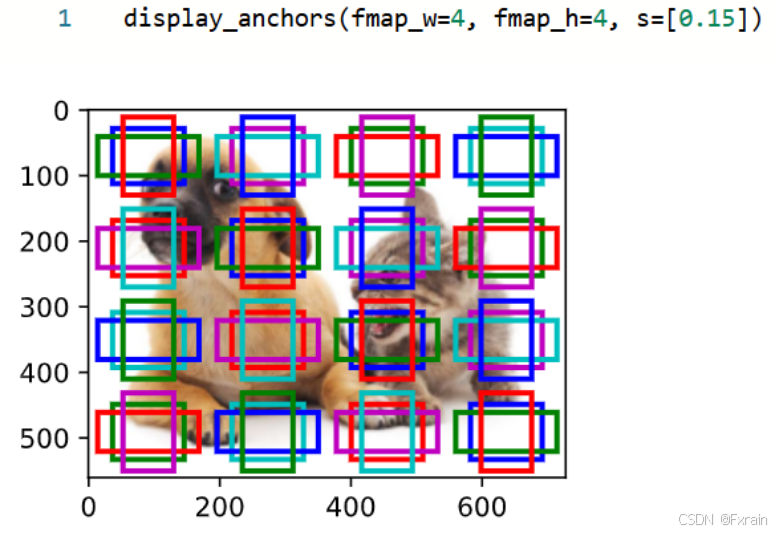
图 15

如图16所示，将特征图的高度和宽度减小一半，然后使用较大的锚框来检测较大的目标。当尺度设置为0.4时，一些锚框将彼此重叠。

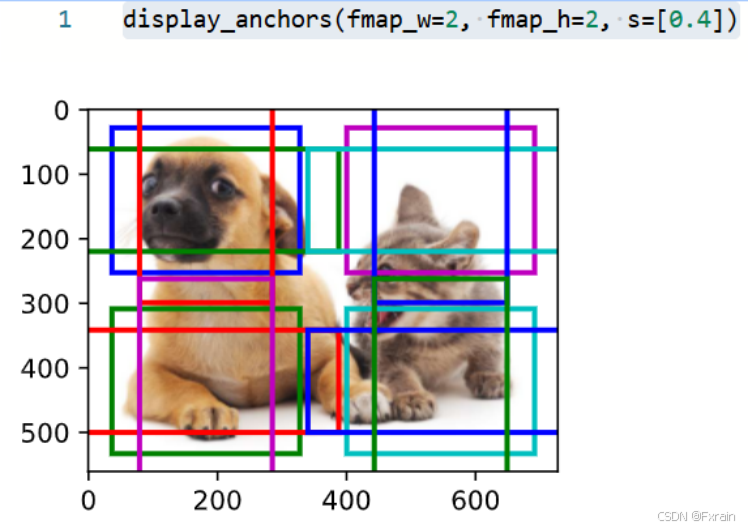
图 16

如图17所示，进一步将特征图的高度和宽度减小一半，然后将锚框的尺度增加到0.8。此时，锚框的中心即是图像的中心。

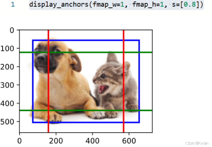
图 17

深度神经网络学习图像特征级别抽象层次，随网络深度的增加而升级。在多尺度目标检测中不同尺度的特征映射对应于不同的抽象层次。因为深度神经网络在学习图像特征时，会随着网络深度的增加而逐步从具体的细节特征转向更高层次的语义信息。深层网络的感受野较大，能够捕捉到更多的上下文信息和语义特征，但分辨率较低，几何细节信息较弱。相反，低层网络的感受野较小，能够保留更多的几何细节信息，但语义信息较弱。深度神经网络通过多个隐藏层的级联，将输入特征连续不断地进行非线性处理，提取和变换出新的特征。在多尺度目标检测中，通常会结合不同尺度的特征映射来提高检测性能。例如，在yolov3中，1/32大小的特征图（深层）具有大的感受野，适合检测大目标；而1/8大小的特征图（较浅层）具有较小的感受野，适合检测小目标。这种多尺度特征的融合能够充分利用不同层次的特征信息，提高检测的准确性和鲁棒性。

给定形状为1×c×h×w1×c×h×w的特征图变量，其中cc、hh和ww分别是特征图的通道数、高度和宽度，实现锚框定义：

（1）定义锚框：首先需要定义一组锚框（anchor boxes），这些锚框通常是预定义的矩形框，它们的大小和比例是固定的。

（2）生成锚框网格：在特征图上生成一个与特征图大小相同的锚框网格。每个位置上的锚框都是基于该位置的中心点生成的。

（3）计算偏移量：对于每个锚框，计算其相对于真实边界框的偏移量。这包括中心点的偏移量（dx, dy）以及宽高的比例变化（dw, dh）。

（4）分类标签：为每个锚框分配一个类别标签，表示它是否包含目标对象。

假设有一个特征图，其形状为 1×c×h×w，并且我们定义了k 个锚框，那么输出的形状如下：锚框类别：形状为 1×(c×k)×h×w。每个位置有 c×k 个值，表示每个位置上的每个锚框的类别。锚框偏移量：形状为 1×(4×k)×h×w。每个位置有 4×k 个值，表示每个位置上的每个锚框的偏移量（dx, dy, dw, dh）。

四、实验小结

在目标检测中，特征提取是基础步骤，它决定了后续分类和定位的准确性。边界框是围绕检测到的物体绘制的矩形，由坐标、宽度和高度定义。锚框是预设的一组不同尺寸和宽高比的框，用于在图像中预测物体的可能位置。评估预测边界框与真实情况匹配程度的指标是交并比（IoU），它测量了预测和实际边界框之间的重叠部分。随着技术的不断进步，目标检测将在更多领域发挥其重要作用，为人们的生活带来更多便利和安全保障。