文章出自：基于 2个Expert 的 MoE 架构分步指南

本篇适合 MoE 架构初学者。文章亮点在于详细拆解 Qwen 3 MoE 架构，并用简单代码从零实现 MoE 路由器、RMSNorm 等核心组件，便于理解内部原理。
该方法适用于需部署高性能、高效率大模型，同时优化计算成本的商业场景。
例如，在智能客服中，不同专家处理特定问题，提升响应速度；或在个性化推荐中，快速生成用户内容。

代码都可以在： GitHub 仓库找到

---

---

1. 前言

阿里巴巴的 Qwen 3 是目前仅次于 DeepSeek 的最佳开源 MoE AI 模型，擅长推理、编码、数学和语言。其顶级版本在 MMLU-Pro、LiveCodeBench 和 AIME 等关键测试中表现出色。

在这篇博客中，我们将使用 2 位专家构建一个微型 Qwen-3 MoE，而不使用面向对象编程（OOP）原则……

因此，我们可以一次查看并理解一个矩阵乘法。

Qwen 3 采用混合专家（MoE）架构构建，每次查询仅激活其 2350 亿参数中的一个子集，从而在不牺牲质量的情况下实现高效率。它还支持高达 128K 标记上下文，处理 119 种语言，并引入了双重“思考”与“非思考”模式，以平衡深度推理和更快的推理。

我们的 Qwen 模型拥有 8 亿参数。

所有代码（理论 + 笔记本）都可以在我的 GitHub 仓库中找到。

正如我所说，我们不会使用面向对象编程（OOP）编码，而只使用简单的 Python 编程。但是，您应该对神经网络和 Transformer 架构有基本的了解。

这是遵循本博客所需的仅有的两个先决条件。

2. 了解 Qwen 3 MoE 架构

我们首先以中级技术人员的身份了解 Qwen MoE 架构，然后使用一个例子“猫坐”来了解它如何通过架构，从而获得清晰的理解。

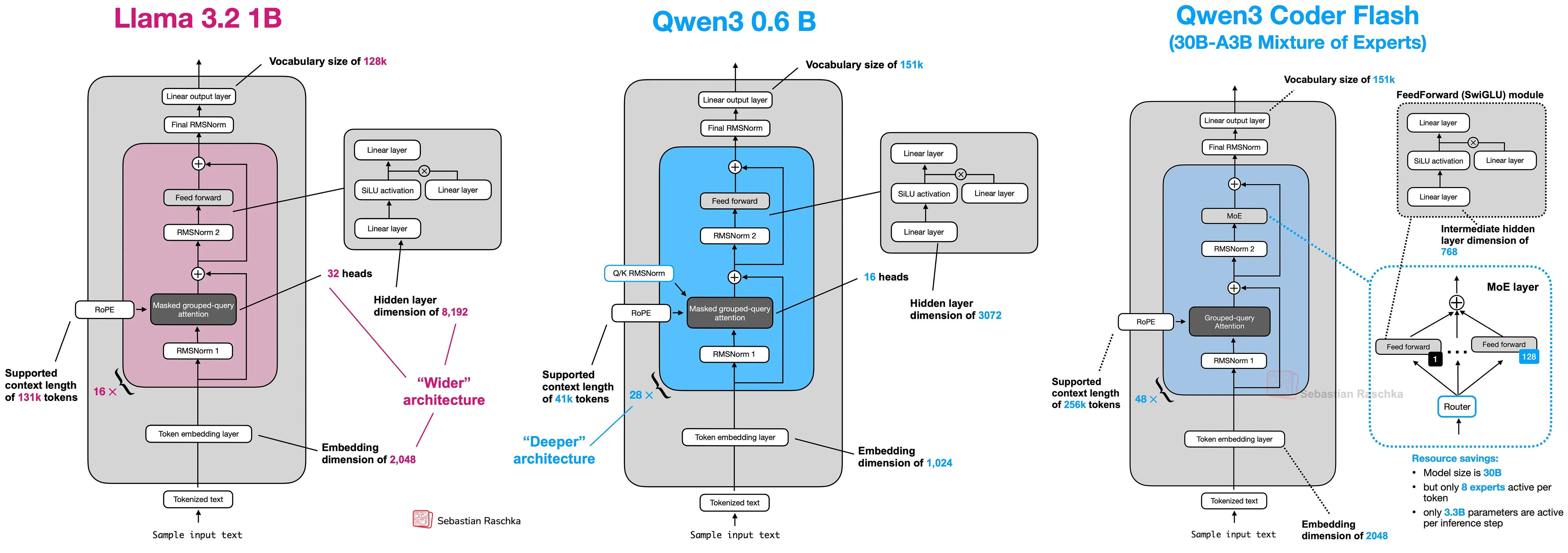
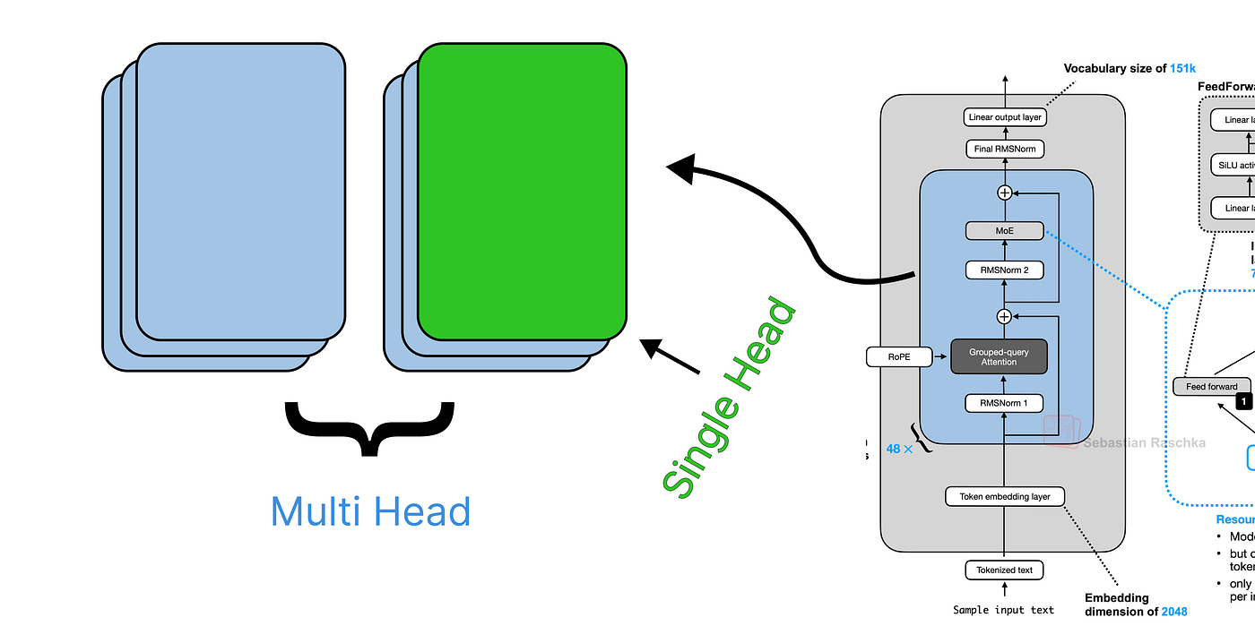
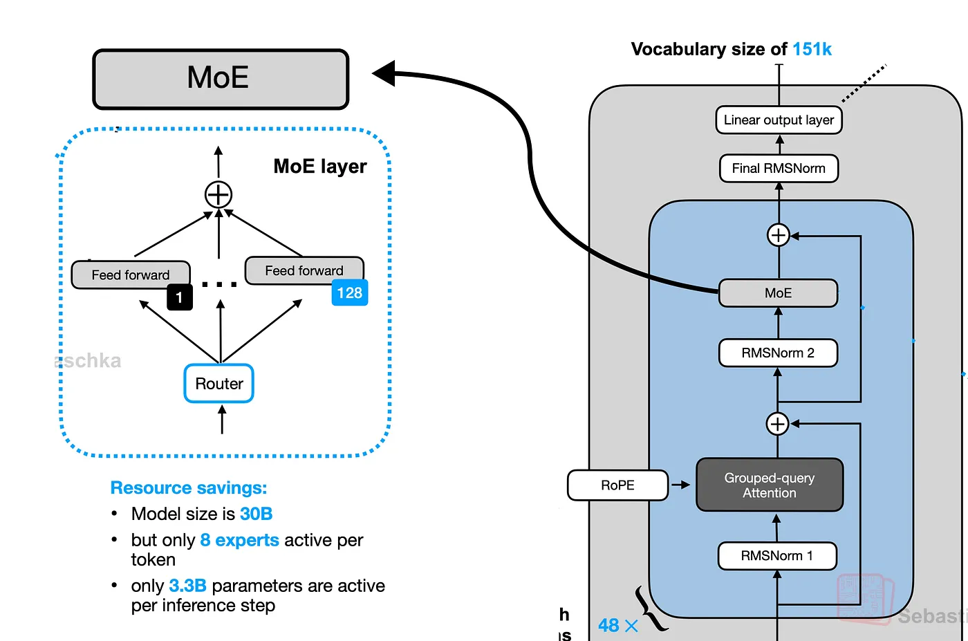
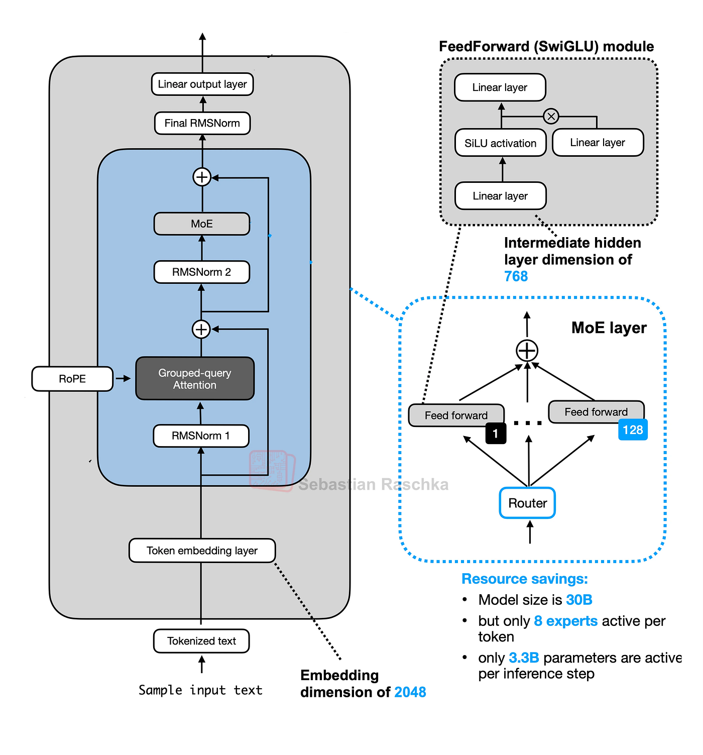
Qwen 3 MoE 架构（来自 Sebastian Raschka）

想象一下你有一项非常艰巨的工作。你不是雇佣一个对所有事情都“略知一二”的人，而是雇佣一个专家团队，每个人都擅长某一项特定技能（比如电工、水管工、油漆工）。你还会雇佣一个经理，他会查看当前任务并将其发送给合适的专家。

AI 模型中的 MoE 有点像这样。MoE 层不是一个试图学习所有内容的庞大神经网络，而是包含：

1. “专家”团队：这些是更小、更专业的神经网络（通常是简单的前馈网络或 MLP）。每个专家可能擅长处理某些类型的信息或模式。
2. “路由器”（经理）：这是另一个小型网络。它的工作是查看输入数据（如一个词或词的一部分），并决定哪些专家最适合立即处理它。

想象一下我们的模型正在处理句子：“The cat sat.”

1. 标记：首先，我们将其分解成小块（标记）：“The”、“cat”、“sat”。
2. 路由器获取标记：MoE 层接收标记 cat（表示为一串数字，一个嵌入向量）。路由器查看这个 cat 向量。
3. 路由器选择：假设我们有 4 位专家（E1、E2、E3、E4）。路由器决定哪些最适合 cat。
4. 也许它认为 E2（可能擅长名词？）和 E4（可能擅长动物概念？）是最佳选择。它为这些选择赋予分数或“权重”（例如，E2 为 70%，E4 为 30%）。

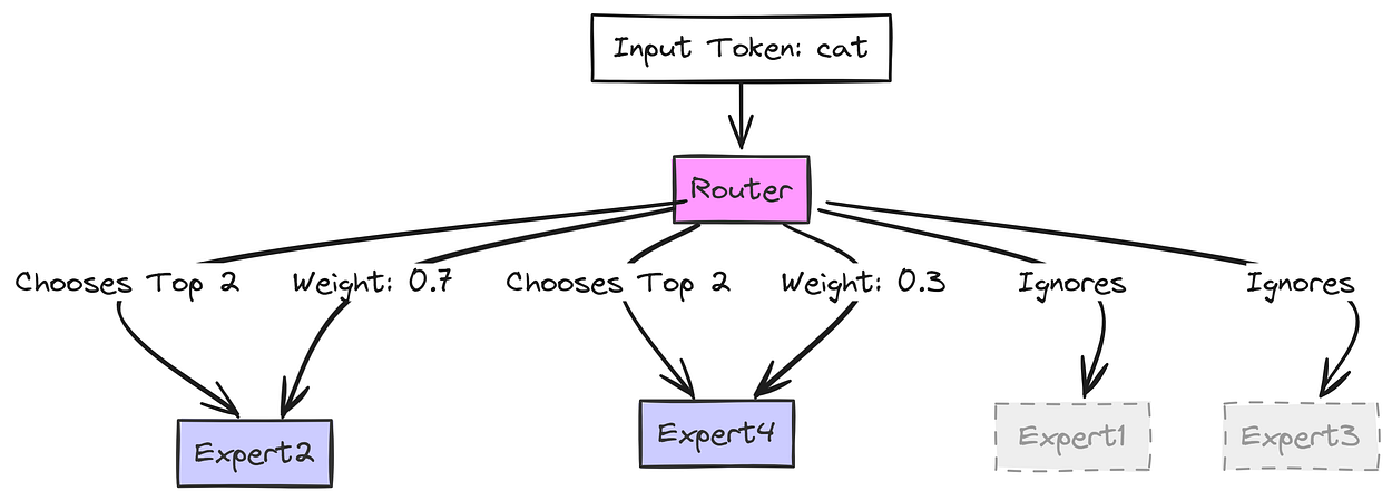
路由器如何决定（由 Fareed Khan 创建）

cat 向量仅发送到 专家 2 和 专家 4。专家 1 和 专家 3 不对此标记执行任何工作，从而节省了计算！E2 处理 cat 并生成其结果（Output_E2）。E4 处理 cat 并生成其结果（Output_E4）。

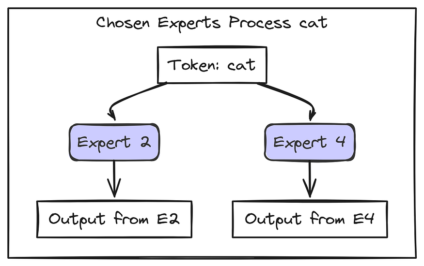
猫词精选专家（由 Fareed Khan 创建）

我们现在使用 路由器 权重组合所选专家的结果：Final_Output = (0.7 * Output_E2) + (0.3 * Output_E4).

这个 Final_Output 是 MoE 层为标记 cat 传递的内容。序列中的每个标记都会发生这种情况！不同的标记可能会被路由到不同的专家。

因此，当我们的模型处理像“The cat sat.”这样的文本时，整个过程如下所示：

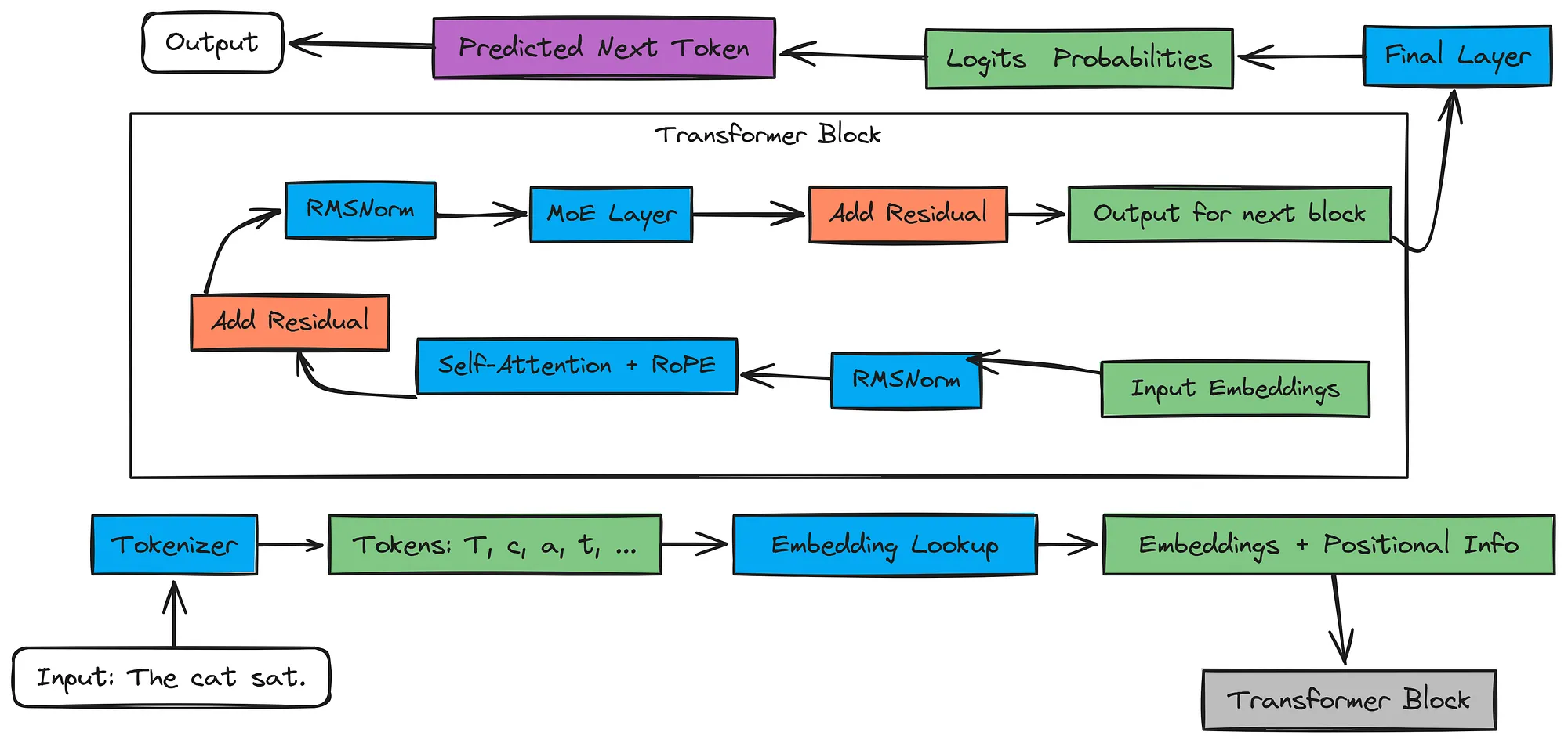
输入文本进入 分词器。分词器创建数字标记 ID。嵌入层将 ID 转换为有意义的数字向量（嵌入）并添加位置信息（稍后在注意力中使用 RoPE）。

这些向量通过多个 Transformer 块。每个块都有：

• 自注意力（其中标记相互关注，由 RoPE 增强）。
• MoE 层（其中 路由器 将标记发送到特定的 专家）。
• 归一化（RMSNorm）和 残差连接 有助于学习。

最后一个块的输出进入 最终层。这一层为我们词汇表中的每个可能的下一个标记生成 Logits（分数）。

我们将 logits 转换为 概率 并 预测下一个标记。

现在我们已经了解了 MoE 如何融入整体，接下来让我们深入了解每个 AI 模型中的较小组件。

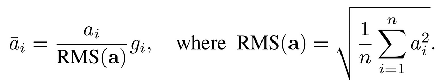
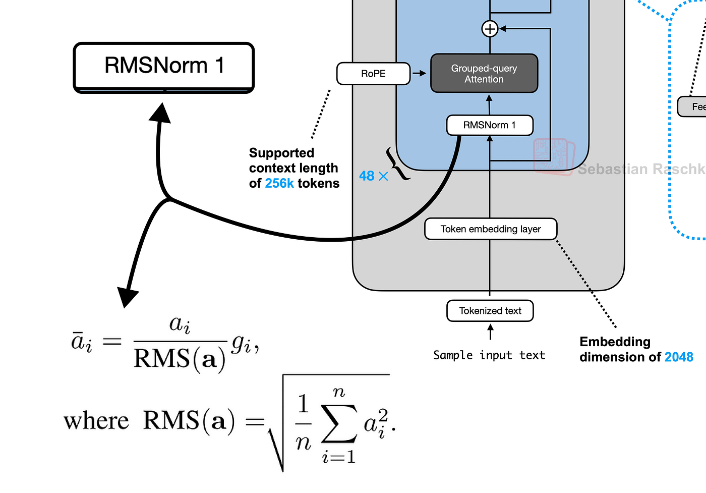
2.1. 使用 RMSNorm 进行预归一化

RMSNorm（均方根归一化）应用于每个 Transformer 子层（注意力或前馈）之前。

它根据输入的均方根缩放输入，而不减去均值（与 LayerNorm 不同）。这有助于稳定训练并在早期保持重要信号的强度，就像在深入研究教科书之前复习关键章节一样。

均方根层归一化论文 (https://arxiv.org/abs/1910.07467)

感兴趣的读者可以在此处探索 RMSNorm 的详细实现。

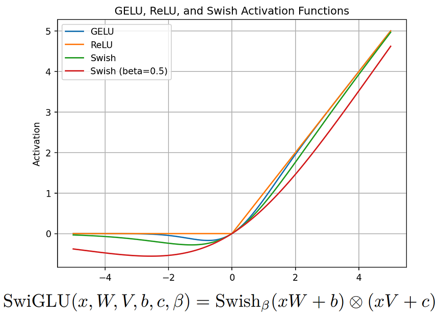
2.2. SwiGLU 激活函数

SwiGLU（Swish + 门控线性单元）增强了模型强调重要特征的能力。

它使用带有 Swish 激活的门控机制，这有助于控制哪些信息通过。

SwiGLU：GLU 变体改进 Transformer (https://kikaben.com/swiglu-2020/)

将其视为一个智能荧光笔，它使关键部分在处理过程中更加突出。

它在 PaLM 中引入，现在用于 LLaMA 3/Qwen 3 以获得更好的性能。有关 SwiGLU 的更多详细信息可以在相关论文中找到。

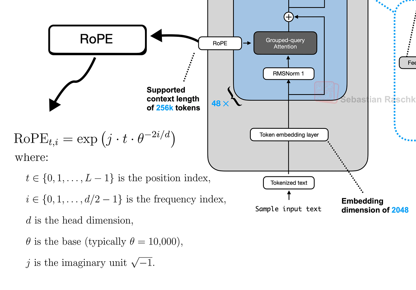
2.3. 旋转位置嵌入 (RoPE)

RoPE 使用正弦函数和旋转扭曲来编码标记位置，使嵌入能够“旋转”以反映相对位置。

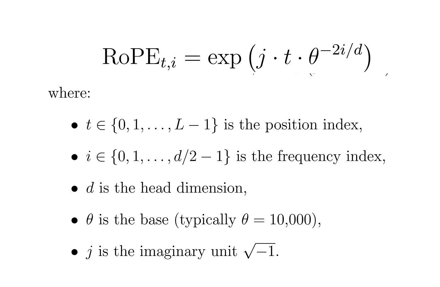
RoPE 公式（由 Fareed Khan 创建）

与固定位置嵌入不同，RoPE 支持更长的上下文和对未见位置的更好泛化。

想象一下学生在一个圆圈中移动，他们的位置会发生变化，但他们的相对距离保持不变。这有助于模型更灵活地跟踪词序。

2.4. 字节对编码 (BPE)

BPE 通过合并频繁的字符对（如“th”、“ing”）来构建标记，使模型能够更有效地处理不常见或新词。

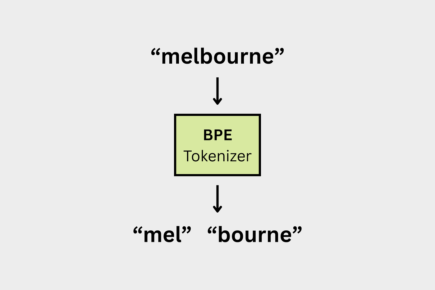
BPE（来自 langformer blog）

Qwen 3 使用 BPE，它倾向于完整的已知词（例如，“hugging”如果在词汇表中，则保持完整）。

而 LLaMA 3 使用 SentencePiece BPE，它可能会将同一个词拆分成多个部分（“hug”+“ging”）。这种差异会影响分词速度以及模型理解文本的方式。

3. 初始化安装

我们将使用少量 Python 库，但最好安装它们以避免遇到**“未找到模块”**错误。

pip install sentencepiece tiktoken torch matplotlib huggingface_hub tokenizers safetensors

安装完所需的库后，我们需要下载 Qwen 3 架构权重和配置文件，这些文件将在本指南中用到。

我们正在针对一个较小的 Qwen 3 MoE 版本，其中包含两个专家，每个专家有 0.8B 参数。必要的文件是 Qwen 3 架构的骨干。有两种方法可以实现这一点。

（选项 1：手动） 转到 Qwen-0.8B-2E HF 目录并手动下载这四个文件中的每一个。

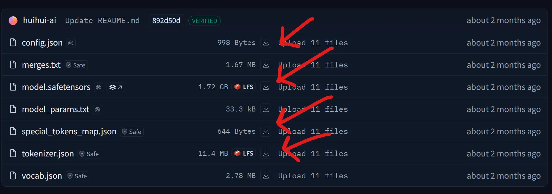
（选项 2：编码） 我们可以使用 huggingface_hub 的 snapshot_download 模块下载 Qwen 3 MoE 模型的整个 Hugging Face 仓库。我们采用这种方法。

from tqdm import tqdm
from huggingface_hub import snapshot_downloadrepo_id = "huihui-ai/Huihui-MoE-0.8B-2E"
local_dir = "Huihui-MoE-0.8B-2E"snapshot_download(repo_id=repo_id,local_dir=local_dir,ignore_patterns=["*.bin"],tqdm_class=tqdm
)

下载所有文件后，我们需要导入将在本博客中使用的库。

import torch
import torch.nn as nnfrom huggingface_hub import snapshot_download
from tokenizers import Tokenizer
from safetensors.torch import load_fileimport json
from pathlib import Path
from tqdm import tqdmimport matplotlib.pyplot as plt

接下来，我们需要了解每个文件的用途。

4. 为什么我们需要模型权重？

由于我们旨在精确复制 Qwen 3 MoE，这意味着我们的输入文本必须产生有意义的输出。
例如，如果我们的输入是**“太阳的颜色是？”** ，输出必须是**“白色”**。
实现这一点需要在大规模数据集上训练我们的 LLM，这需要高计算能力，对我们来说是不可行的。

然而，阿里巴巴已经公开了他们的 Qwen 3 架构文件，或者更复杂地说，他们预训练的权重供使用。我们刚刚下载了这些文件，这使我们能够复制他们的架构，而无需训练或大量数据集。一切都已准备就绪，我们只需在正确的位置使用正确的组件。

tokenizer.json — Qwen 3 使用字节对编码（BPE），Andrej Karpathy 有一个非常简洁的 BPE 实现。

tokenizer_path = Path("Huihui-MoE-0.8B-2E/tokenizer.json")tokenizer = Tokenizer.from_file(str(tokenizer_path))with open("Huihui-MoE-0.8B-2E/special_tokens_map.json", "r") as f:special_tokens_map = json.load(f)print(f"Special tokens from file: {special_tokens_map}")

Special tokens from file: {
'additional_special_tokens': ['<|im_start|>',
'<|im_end|>', '<|object_ref_start|>', '<|object_ref_end|>', '<|box_start|>'
...
}

这些特殊标记将用于包装我们的提示，以指导我们的 Qwen 3 架构如何响应我们的查询。

# We'll follow the encode -> decode pattern to ensure it works correctly.
prompt = "The only thing I know is that I know"# .encode() returns an Encoding object, we access the token IDs via .ids
encoded = tokenizer.encode(prompt)
print(f"\nOriginal prompt: '{prompt}'")
print(f"Encoded token IDs: {encoded.ids}")# .decode() converts the token IDs back to a string.
decoded = tokenizer.decode(encoded.ids)
print(f"Decoded back to text: '{decoded}'")# Verify the vocabulary size
vocab_size = tokenizer.get_vocab_size()
print(f"\nTokenizer vocabulary size: {vocab_size}")#### OUTPUT ####
Original prompt: 'The only thing I know is that I know'
Encoded token IDs: [785, 1172, 3166, 358, 1414, 374, 429, 358, 1414]
Decoded back to text: 'The only thing I know is that I know'
Tokenizer vocabulary size: 151669

词汇量大小表示训练数据中唯一字符的数量。tokenizer 的类型是一个字典。

# Get the vocabulary as a dictionary: {token_string: token_id}
vocab = tokenizer.get_vocab()# Display a slice of the vocabulary for inspection (tokens 5600 to 5609)
sample_vocab_slice = list(vocab.items())[5600:5610]
sample_vocab_slice#### OUTPUT ####
[('íĮIJ', 129382),('ĠBrands', 54232),('Ġincorporates', 51824),('à¸ŀระราà¸Ĭ', 132851),('ĉResource', 79487),('ĠĠĠĠĉĠ', 80840),('hover', 17583),('Movement', 38050),('解åĨ³äºĨ', 105826),('ĠonBackPressed', 70609)]

当我们从中打印 10 个随机项时，您会看到使用 BPE 算法形成的字符串。键表示来自 BPE 训练的字节序列，而值表示基于频率的合并排名。

config.json — 包含各种参数值，例如：

# Define the path to the configuration file.
config_path = Path("Huihui-MoE-0.8B-2E/config.json")# Open and load the JSON file into a Python dictionary.
with open(config_path, "r") as f:config = json.load(f)# Print the configuration to see all the parameters.
# This gives us a complete overview of the model we're about to build.
print(json.dumps(config, indent=4))#### OUTPUT ####
{"architectures": ["Qwen3MoeForCausalLM"],"attention_bias": false,"attention_dropout": 0.0,"bos_token_id": 151643,"decoder_sparse_step": 1,"eos_token_id": 151645,"head_dim": 128,"hidden_act": "silu",..."transformers_version": "4.52.4","use_cache": true,"use_sliding_window": false,"vocab_size": 151936
}

这些值将通过指定注意力头数、嵌入向量维度、专家数量等细节来帮助我们复制 Qwen-3 架构。

让我们存储这些值，以便以后使用。

# --- Main Architecture Parameters ---
# Extract model hyperparameters from the config dictionary.# Embedding dimension (hidden size of the model)
dim = config["hidden_size"]
# Number of transformer layers
n_layers = config["num_hidden_layers"]
# Number of attention heads
n_heads = config["num_attention_heads"]
# Number of key/value heads (for grouped-query attention)
n_kv_heads = config["num_key_value_heads"]
# Vocabulary size
vocab_size = config["vocab_size"]
# RMSNorm epsilon value for numerical stability
norm_eps = config["rms_norm_eps"]
# Rotary positional embedding theta parameter
rope_theta = torch.tensor(config["rope_theta"])
# Dimension of each attention head
head_dim = config["head_dim"]  # For attention calculations# --- Mixture-of-Experts (MoE) Specific Parameters ---
# Number of experts in the MoE layer
num_experts = config["num_experts"]
# Number of experts selected per token by the router
num_experts_per_tok = config["num_experts_per_tok"]
# Intermediate size of the MoE feed-forward network
moe_intermediate_size = config["moe_intermediate_size"]

model.safetensors — 包含 Qwen 0.8B 2 专家模型的学习参数（权重）。这些参数包含模型如何理解和处理语言的信息，例如它如何表示标记、计算注意力、执行专家选择以及归一化其输出。

model_weights_path = Path("Huihui-MoE-0.8B-2E/model.safetensors")model_weights = load_file(model_weights_path)print("First 20 keys in model_weights:")
print(json.dumps(list(model_weights.keys())[:20], indent=4))

OUTPUT：

["model.embed_tokens.weight","model.layers.0.input_layernorm.weight","model.layers.0.mlp.experts.0.down_proj.weight","model.layers.0.mlp.experts.0.gate_proj.weight","model.layers.0.mlp.experts.0.up_proj.weight","model.layers.0.mlp.experts.1.down_proj.weight",..."model.layers.1.mlp.experts.0.gate_proj.weight","model.layers.1.mlp.experts.0.up_proj.weight"...
]

如果您熟悉 Transformer 架构，您就会知道查询、键矩阵等等。稍后，我们将使用这些层/权重来创建这些矩阵以及 Qwen 3 MoE 架构中的 MoE 组件。

现在我们有了分词器模型、包含权重的架构模型和配置参数，让我们开始从头开始编码我们自己的 Qwen 3 MoE。

5. Tokenized文本

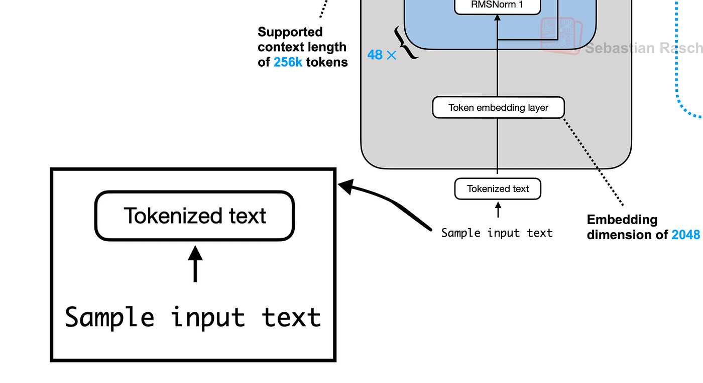
标记化输入文本（由 Fareed Khan 创建）

第一步是将我们的输入文本转换为标记。Qwen 3 使用带有特殊标记（如 <|im_start|> 和 <|im_end|>）的特定聊天模板来构建对话。这有助于模型区分用户查询和它自己的响应。

prompt = "The only thing I know is that I know"im_start_id = tokenizer.token_to_id("<|im_start|>")
im_end_id = tokenizer.token_to_id("<|im_end|>")
newline_id = tokenizer.encode("\n").ids[0]
user_ids = tokenizer.encode
````python
assistant_ids = tokenizer.encode("assistant").ids
prompt_ids = tokenizer.encode(prompt).idsprefix_ids = [im_start_id] + user_ids + [newline_id]
suffix_ids = [im_end_id, newline_id, im_start_id] + assistant_ids + [newline_id]
tokens_list = prefix_ids + prompt_ids + suffix_idstokens = torch.tensor(tokens_list)print(f"Final combined token IDs: {tokens}")prompt_split_as_tokens = [tokenizer.decode([token.item()]) for token in tokens]
print(f"\nPrompt split into tokens: {prompt_split_as_tokens}")

OUTPUT：

Final combined token IDs: tensor([151644,    872,  ... , 8])
Prompt split into tokens: ['', 'user', '\n', 'The', ..., '\n']

我们现在已经将提示转换为一个包含 17 个标记的结构化列表，准备好供模型使用。

6. 创建令牌嵌入层

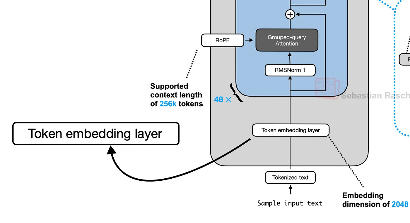
生成标记化文本的嵌入（由 Fareed Khan 创建）

嵌入是一个密集向量，用于在高维空间中表示标记的含义。我们的 17 个标记的输入向量需要转换为 [17, 1024] 的张量，其中 1024 (dim) 是嵌入维度。

embedding_layer = nn.Embedding(vocab_size, dim)embedding_layer.weight.data.copy_(model_weights["model.embed_tokens.weight"])token_embeddings_unnormalized = embedding_layer(tokens).to(torch.bfloat16)print("Shape of the token embeddings:", token_embeddings_unnormalized.shape)

OUTPUT

Shape of the token embeddings: torch.Size([17, 1024])

这些嵌入未归一化，如果我们不进行归一化，将产生严重影响。在下一节中，我们将对输入向量执行归一化。

7. 使用 RMSNorm 进行规范化

我们将定义 rms_norm 函数，它根据输入的均方根值缩放输入。这是我们 Transformer 层中的第一个预归一化步骤。

均方根层归一化论文 (https://arxiv.org/abs/1910.07467)

def rms_norm(tensor, norm_weights):input_dtype = tensor.dtypetensor_float = tensor.to(torch.float32)variance = tensor_float.pow(2).mean(-1, keepdim=True)normalized_tensor = tensor_float * torch.rsqrt(variance + norm_eps)return (normalized_tensor * norm_weights).to(input_dtype)

我们将使用 layers_0 的注意力权重来归一化我们未归一化的嵌入。使用 layer_0 的原因是，我们现在正在创建 Qwen 3 架构的第一层。

token_embeddings_normalized = rms_norm(token_embeddings_unnormalized,model_weights["model.layers.0.input_layernorm.weight"]
)
print("Shape of the normalized token embeddings:", token_embeddings_normalized.shape)

Shape of the normalized token embeddings: torch.Size([17, 1024])

形状保持不变，但值现在已归一化，并准备好用于注意力机制。

8. 分组查询注意力 (GQA)

接下来，我们生成查询 (Q)、键 (K) 和值 (V) 向量。预训练权重存储在大的组合矩阵中。我们需要重塑它们以分离出我们 16 个注意力头的每个头的权重。

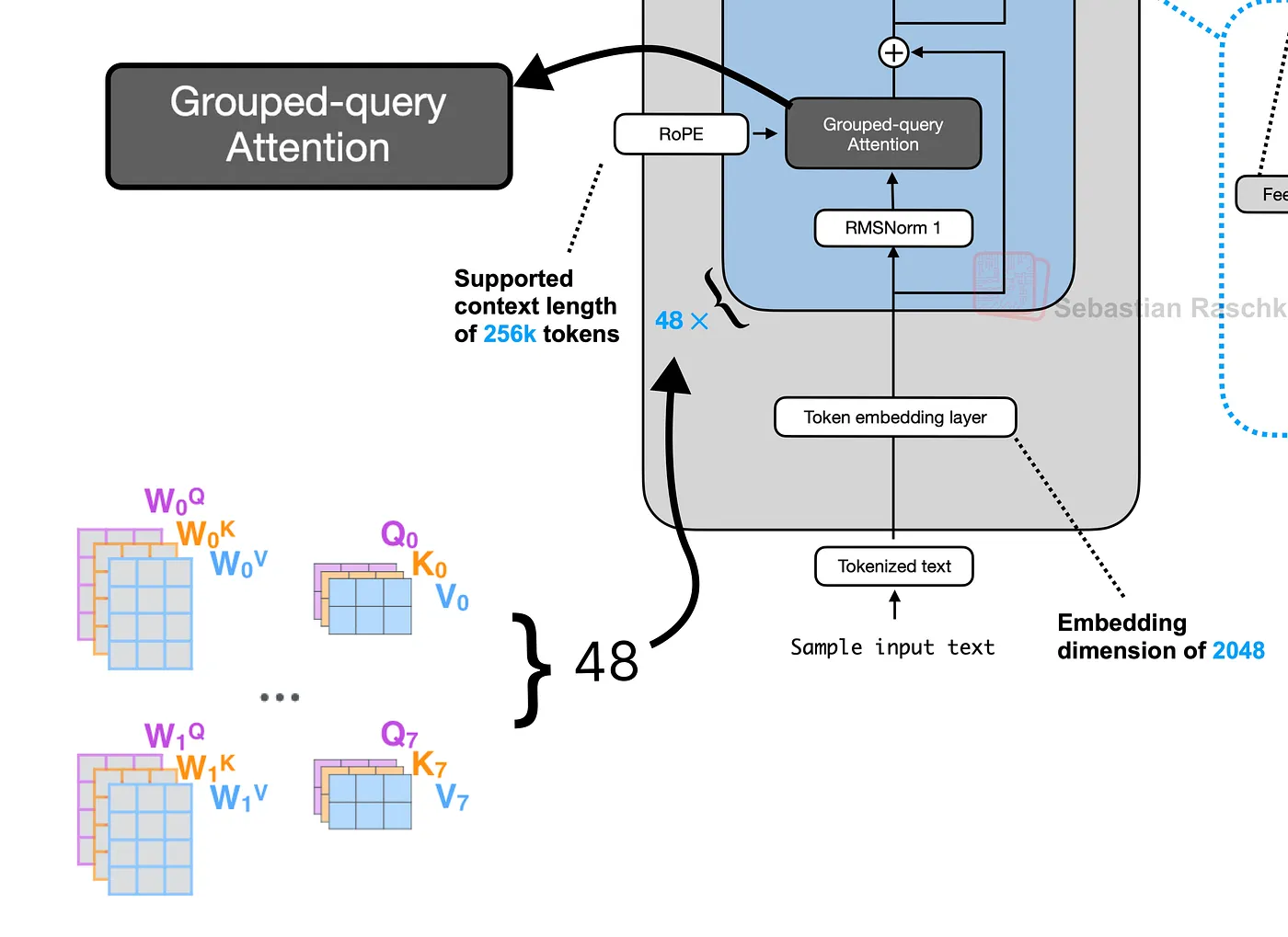
分组查询注意力 (GQA)（由 Fareed Khan 创建）

该模型使用一种称为分组查询注意力 (GQA) 的优化，其中多个查询头 (16) 共享少量键和值头 (8)。这在不显著降低性能的情况下减少了计算负载。

q_layer0 = model_weights["model.layers.0.self_attn.q_proj.weight"]
q_layer0 = q_layer0.view(n_heads, head_dim, dim)k_layer0 = model_weights["model.layers.0.self_attn.k_proj.weight"]
k_layer0 = k_layer0.view(n_kv_heads, head_dim, dim)v_layer0 = model_weights["model.layers.0.self_attn.v_proj.weight"]
v_layer0 = v_layer0.view(n_kv_heads, head_dim, dim)

现在，让我们通过将归一化嵌入乘以头的权重来计算第一个头的 Q、K 和 V 向量。

q_layer0_head0 = q_layer0[0]
k_layer0_head0 = k_layer0[0]
v_layer0_head0 = v_layer0[0]q_per_token = torch.matmul(token_embeddings_normalized, q_layer0_head0.T)
k_per_token = torch.matmul(token_embeddings_normalized, k_layer0_head0.T)
v_per_token = torch.matmul(token_embeddings_normalized, v_layer0_head0.T)print("Shape of Query vectors per token:", q_per_token.shape)

Shape of Query vectors per token: torch.Size([17, 128])

我们 17 个标记中的每个标记现在都有一个 128 维的 Q、K 和 V 向量，用于第一个头。

9. 使用 RoPE

这些向量尚未知道它们的位置。我们将使用 RoPE 通过“旋转”它们来注入这些信息。为了提高效率，我们可以预先计算所有可能位置（直到最大序列长度）的旋转角度。

RoPE 实现（由 Fareed Khan 创建）

这将创建一个旋转矩阵的查找表，表示为复数。

max_seq_len = config["max_position_embeddings"]
freqs = 1.0 / (rope_theta ** (torch.arange(0, head_dim, 2) / head_dim))
t = torch.arange(max_seq_len)
freqs_for_each_token = torch.outer(t, freqs)freqs_cis = torch.polar(torch.ones_like(freqs_for_each_token), freqs_for_each_token)

这个 freqs_cis 张量现在包含将执行旋转的复数。我们可以可视化单个标记的旋转，以查看每个 2D 维度对如何以不同的角度旋转。

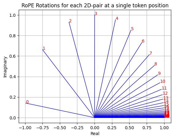
单个标记位置上每个 2D 对的 RoPE 旋转（由 Fareed Khan 创建）

现在，我们将这些旋转应用于我们的 Q 和 K 向量。通过将向量视为复数并执行逐元素乘法来执行旋转。

freqs_cis_for_tokens = freqs_cis[:len(tokens)]q_per_token_as_complex_numbers = torch.view_as_complex(q_per_token.float().view(q_per_token.shape[0], -1, 2))
q_per_token_rotated_complex = q_per_token_as_complex_numbers * freqs_cis_for_tokens
q_per_token_rotated = torch.view_as_real(q_per_token_rotated_complex).view(q_per_token.shape)k_per_token_as_complex_numbers = torch.view_as_complex(k_per_token.float().view(k_per_token.shape[0], -1, 2))
k_per_token_rotated_complex = k_per_token_as_complex_numbers * freqs_cis_for_tokens
k_per_token_rotated = torch.view_as_real(k_per_token_rotated_complex).view(k_per_token.shape)print("Shape of rotated Query vectors:", q_per_token_rotated.shape)

Shape of rotated Query vectors: torch.Size([17, 128])

10. 计算注意力分数

现在我们通过计算查询和键矩阵的点积来计算注意力分数。这将创建一个 [17, 17] 矩阵，显示每个标记应该“关注”其他每个标记的程度。

我们通过头维度的平方根来缩放分数，以稳定训练。

qk_per_token = torch.matmul(q_per_token_rotated, k_per_token_rotated.T)qk_per_token_scaled = qk_per_token / (head_dim**0.5)

我们可以将这些原始分数可视化为热图。

qk_per_token = torch.matmul(q_per_token_rotated, k_per_token_rotated.T)qk_per_token_scaled = qk_per_token / (head_dim**0.5)def display_qk_heatmap(qk_matrix, title="Attention Heatmap"):_, ax = plt.subplots()im = ax.imshow(qk_matrix.to(torch.float32).detach(), cmap='viridis')ax.set_xticks(range(len(prompt_split_as_tokens)))ax.set_yticks(range(len(prompt_split_as_tokens)))ax.set_xticklabels(prompt_split_as_tokens, rotation=90)ax.set_yticklabels(prompt_split_as_tokens)ax.figure.colorbar(im, ax=ax)plt.title(title)plt.show()display_qk_heatmap(qk_per_token_scaled, title="Raw Attention Scores (Before Masking)")

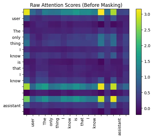
原始注意力分数（掩码前）

为了防止标记在这种自回归模型中“看到”未来，我们应用因果掩码。这将矩阵上三角形中的所有分数设置为负无穷大，因此它们在 softmax 函数后变为零。

mask = torch.full((len(tokens), len(tokens)), float("-inf"))
mask = torch.triu(mask, diagonal=1)qk_per_token_masked = qk_per_token_scaled + mask

如果我们看看掩码矩阵的样子。

print(mask)

tensor([[0., -inf, -inf, -inf, -inf, -inf, -inf, -inf, -inf, -inf, -inf, -inf, -inf, -inf, -inf, -inf, -inf],[0., 0., -inf, -inf, -inf, -inf, -inf, -inf, -inf, -inf, -inf, -inf, -inf, -inf, -inf, -inf, -inf],[0., 0., 0., -inf, -inf, -inf, -inf, -inf, -inf, -inf, -inf, -inf, -inf, -inf, -inf, -inf, -inf],[0., 0., 0., 0., -inf, -inf, -inf, -inf, -inf, -inf, -inf, -inf, -inf, -inf, -inf, -inf, -inf],[0., 0., 0., 0., 0., -inf, -inf, -inf, -inf, -inf, -inf, -inf, -inf, -inf, -inf, -inf, -inf],[0., 0., 0., 0., 0., 0., -inf, -inf, -inf, -inf, -inf, -inf, -inf, -inf, -inf, -inf, -inf],[0., 0., 0., 0., 0., 0., 0., -inf, -inf, -inf, -inf, -inf, -inf, -inf, -inf, -inf, -inf],[0., 0., 0., 0., 0., 0., 0., 0., -inf, -inf, -inf, -inf, -inf, -inf, -inf, -inf, -inf],[0., 0., 0., 0., 0., 0., 0., 0., 0., -inf, -inf, -inf, -inf, -inf, -inf, -inf, -inf],[0., 0., 0., 0., 0., 0., 0., 0., 0., 0., -inf, -inf, -inf, -inf, -inf, -inf, -inf],[0., 0., 0., 0., 0., 0., 0., 0., 0., 0., 0., -inf, -inf, -inf, -inf, -inf, -inf],[0., 0., 0., 0., 0., 0., 0., 0., 0., 0., 0., 0., -inf, -inf, -inf, -inf, -inf],[0., 0., 0., 0., 0., 0., 0., 0., 0., 0., 0., 0., 0., -inf, -inf, -inf, -inf],[0., 0., 0., 0., 0., 0., 0., 0., 0., 0., 0., 0., 0., 0., -inf, -inf, -inf],[0., 0., 0., 0., 0., 0., 0., 0., 0., 0., 0., 0., 0., 0., 0., -inf, -inf],[0., 0., 0., 0., 0., 0., 0., 0., 0., 0., 0., 0., 0., 0., 0., 0., -inf],[0., 0., 0., 0., 0., 0., 0., 0., 0., 0., 0., 0., 0., 0., 0., 0., 0.]])

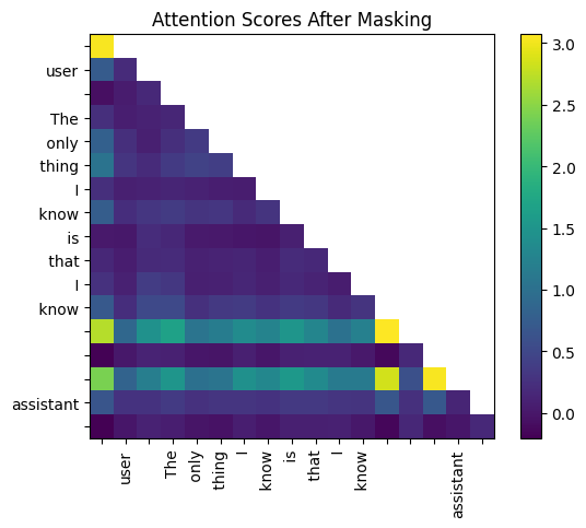
掩码后的注意力分数

最后，我们应用 softmax 函数将这些分数转换为概率（注意力权重），并将它们乘以值矩阵。这将产生值的加权和，为我们提供此注意力头的最终输出。

qk_per_token_after_masking_after_softmax = torch.nn.functional.softmax(qk_per_token_masked.float(), dim=1).to(torch.bfloat16)qkv_attention = torch.matmul(qk_per_token_after_masking_after_softmax, v_per_token)print("Shape of the final attention output for Head 0:", qkv_attention.shape)

Shape of the final attention output for Head 0: torch.Size([17, 128])

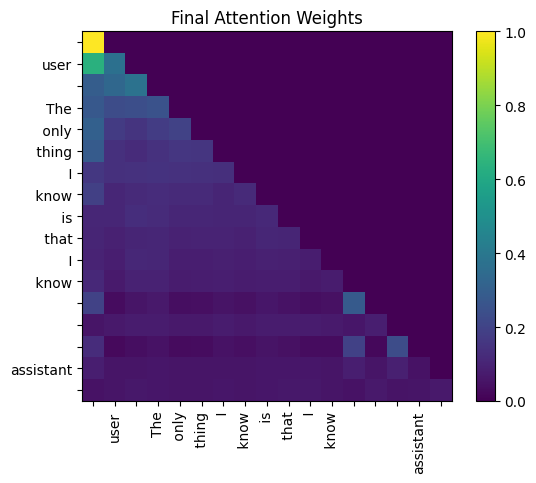
最终注意力权重（由 Fareed Khan 创建）

输出是一个新的 [17, 128] 张量，其中每个标记的向量现在包含来自所有先前标记的上下文信息。

11. 实现多头注意力

我们现在在一个循环中对所有 16 个头重复自注意力过程。每个头的输出（[17, 128] 张量）被收集到一个列表中。

多头注意力（由 Fareed Khan 创建）

qkv_attention_store = []for head in range(n_heads):q_layer0_head = q_layer0[head]k_layer0_head = k_layer0[head // (n_heads // n_kv_heads)]v_layer0_head = v_layer0[head // (n_heads // n_kv_heads)]q_per_token = torch.matmul(token_embeddings_normalized, q_layer0_head.T)k_per_token = torch.matmul(token_embeddings_normalized, k_layer0_head.T)v_per_token = torch.matmul(token_embeddings_normalized, v_layer0_head.T)q_per_token_split_into_pairs = q_per_token.float().view(q_per_token.shape[0], -1, 2)q_per_token_as_complex_numbers = torch.view_as_complex(q_per_token_split_into_pairs)q_per_token_as_complex_numbers_rotated = q_per_token_as_complex_numbers * freqs_cis_for_tokensq_per_token_split_into_pairs_rotated = torch.view_as_real(q_per_token_as_complex_numbers_rotated)q_per_token_rotated = q_per_token_split_into_pairs_rotated.view(q_per_token.shape)k_per_token_split_into_pairs = k_per_token.float().view(k_per_token.shape[0], -1, 2)k_per_token_as_complex_numbers = torch.view_as_complex(k_per_token_split_into_pairs)k_per_token_as_complex_numbers_rotated = k_per_token_as_complex_numbers * freqs_cis_for_tokensk_per_token_split_into_pairs_rotated = torch.view_as_real(k_per_token_as_complex_numbers_rotated)k_per_token_rotated = k_per_token_split_into_pairs_rotated.view(k_per_token.shape)qk_per_token = torch.matmul(q_per_token_rotated, k_per_token_rotated.T) / (head_dim**0.5)qk_per_token_masked = qk_per_token + maskqk_per_token_after_masking_after_softmax = torch.nn.functional.softmax(qk_per_token_masked.float(), dim=1).to(torch.bfloat16)qkv_attention = torch.matmul(qk_per_token_after_masking_after_softmax, v_per_token)qkv_attention_store.append(qkv_attention)

循环结束后，我们将 16 个头的输出连接成一个大小为 [17, 2048] 的大张量。然后使用输出权重矩阵 o_proj 将其投影回模型的维度 (1024)。

stacked_qkv_attention = torch.cat(qkv_attention_store, dim=-1)w_layer0 = model_weights["model.layers.0.self_attn.o_proj.weight"]embedding_delta = torch.matmul(stacked_qkv_attention, w_layer0.T)

结果 embedding_delta 被加回到层的原始输入中。这是第一个残差连接，这是一项关键技术，通过允许梯度更轻松地流动，有助于训练非常深的神经网络。

embedding_after_attention = token_embeddings_unnormalized + embedding_delta

12. 专家混合 (MoE) 块

这是 Transformer 块的第二个子层。首先，我们对其输入应用预归一化。

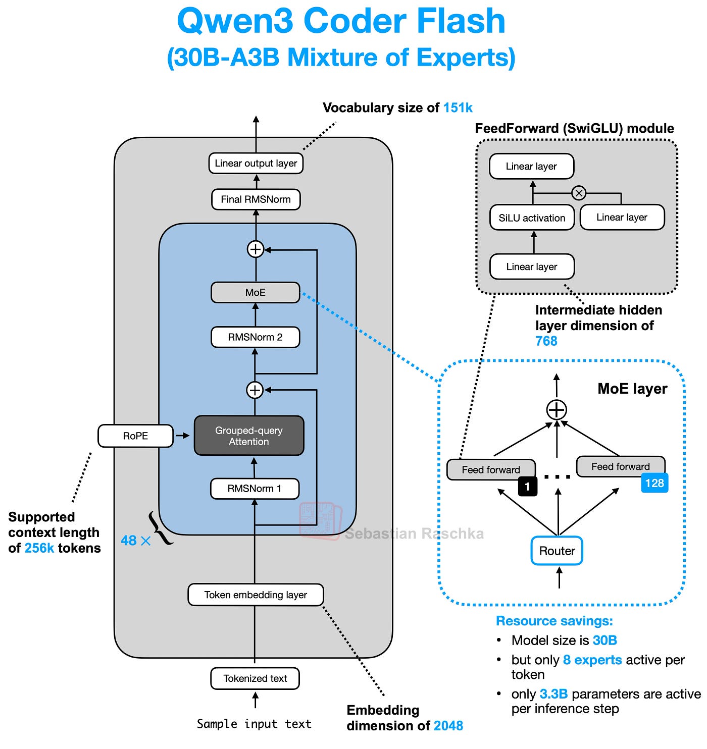
Qwen 3 MoE 层（由 Fareed Khan 创建）

embedding_after_attention_normalized = rms_norm(embedding_after_attention,model_weights["model.layers.0.post_attention_layernorm.weight"]
)

接下来，路由器（一个简单的线性层）计算分数以确定每个标记应该发送到两个专家中的哪一个。

gate = model_weights["model.layers.0.mlp.gate.weight"]
router_logits = torch.matmul(embedding_after_attention_normalized, gate.T)routing_weights = torch.nn.functional.softmax(router_logits.float(), dim=1).to(torch.bfloat16)
routing_expert_indices = torch.argmax(routing_weights, dim=1)print("Router logits shape:", router_logits.shape)
print("Expert chosen for each of the 17 tokens:", routing_expert_indices)

Router logits shape: torch.Size([17, 2])
Expert chosen for each of the 17 tokens: tensor([1, 1, 1, 1, 1, 1, 1, 1, 1, 1, 1, 1, 1, 1, 1, 1, 1])

在这种情况下，路由器决定将所有 17 个标记发送给专家 1。我们现在通过每个标记选择的专家的前馈网络 (FFN) 处理每个标记的嵌入，并根据路由器的概率加权组合结果。

expert0_w1 = model_weights["model.layers.0.mlp.experts.0.gate_proj.weight"]
expert0_w2 = model_weights["model.layers.0.mlp.experts.0.down_proj.weight"]
expert0_w3 = model_weights["model.layers.0.mlp.experts.0.up_proj.weight"]expert1_w1 = model_weights["model.layers.0.mlp.experts.1.gate_proj.weight"]
expert1_w2 = model_weights["model.layers.0.mlp.experts.1.down_proj.weight"]
expert1_w3 = model_weights["model.layers.0.mlp.experts.1.up_proj.weight"]final_expert_output = torch.zeros_like(embedding_after_attention_normalized)for i, token_embedding in enumerate(embedding_after_attention_normalized):chosen_expert_index = routing_expert_indices[i]if chosen_expert_index == 0:w1, w2, w3 = expert0_w1, expert0_w2, expert0_w3else:w1, w2, w3 = expert1_w1, expert1_w2, expert1_w3silu_output = torch.nn.functional.silu(torch.matmul(token_embedding, w1.T))gated_output = silu_output * torch.matmul(token_embedding, w3.T)expert_output = torch.matmul(gated_output, w2.T)final_expert_output[i] = expert_output * routing_weights[i, chosen_expert_index]

最后，我们将 MoE 块的输出添加回注意力块的输出。这是第二个残差连接，完成了 Transformer 层。

layer_0_embedding = embedding_after_attention + final_expert_output

13. 合并层

现在我们有了所有组件，我们可以通过遍历所有 28 层来构建完整的模型。

一层的输出成为下一层的输入。

合并一切（来自 Sebastian Raschka）

final_embedding = token_embeddings_unnormalizedfor layer in range(n_layers):attention_input = rms_norm(final_embedding, model_weights[f"model.layers.{layer}.input_layernorm.weight"])q_layer = model_weights[f"model.layers.{layer}.self_attn.q_proj.weight"].view(n_heads, head_dim, dim)k_layer = model_weights[f"model.layers.{layer}.self_attn.k_proj.weight"].view(n_kv_heads, head_dim, dim)v_layer = model_weights[f"model.layers.{layer}.self_attn.v_proj.weight"].view(n_kv_heads, head_dim, dim)w_layer = model_weights[f"model.layers.{layer}.self_attn.o_proj.weight"]qkv_attention_store = []for head in range(n_heads):q_layer_head = q_layer[head]k_layer_head = k_layer[head // (n_heads // n_kv_heads)]v_layer_head = v_layer[head // (n_heads // n_kv_heads)]q_per_token = torch.matmul(attention_input, q_layer_head.T)k_per_token = torch.matmul(attention_input, k_layer_head.T)v_per_token = torch.matmul(attention_input, v_layer_head.T)q_per_token_rotated = torch.view_as_real(torch.view_as_complex(q_per_token.float().view(q_per_token.shape[0], -1, 2)) * freqs_cis_for_tokens).view(q_per_token.shape)k_per_token_rotated = torch.view_as_real(torch.view_as_complex(k_per_token.float().view(k_per_token.shape[0], -1, 2)) * freqs_cis_for_tokens).view(k_per_token.shape)qk_per_token = torch.matmul(q_per_token_rotated, k_per_token_rotated.T) / (head_dim**0.5)qk_per_token_masked = qk_per_token + maskqk_per_token_after_masking_after_softmax = torch.nn.functional.softmax(qk_per_token_masked.float(), dim=1).to(torch.bfloat16)qkv_attention = torch.matmul(qk_per_token_after_masking_after_softmax, v_per_token)qkv_attention_store.append(qkv_attention)stacked_qkv_attention = torch.cat(qkv_attention_store, dim=-1)embedding_delta = torch.matmul(stacked_qkv_attention, w_layer.T)embedding_after_attention = final_embedding + embedding_deltamoe_input = rms_norm(embedding_after_attention, model_weights[f"model.layers.{layer}.post_attention_layernorm.weight"])gate = model_weights[f"model.layers.{layer}.mlp.gate.weight"]router_logits = torch.matmul(moe_input, gate.T)routing_weights = torch.nn.functional.softmax(router_logits.float(), dim=1).to(torch.bfloat16)routing_expert_indices = torch.argmax(routing_weights, dim=1)final_expert_output = torch.zeros_like(moe_input)expert0_w1 = model_weights[f"model.layers.{layer}.mlp.experts.0.gate_proj.weight"]expert0_w2 = model_weights[f"model.layers.{layer}.mlp.experts.0.down_proj.weight"]expert0_w3 = model_weights[f"model.layers.{layer}.mlp.experts.0.up_proj.weight"]expert1_w1 = model_weights[f"model.layers.{layer}.mlp.experts.1.gate_proj.weight"]expert1_w2 = model_weights[f"model.layers.{layer}.mlp.experts.1.down_proj.weight"]expert1_w3 = model_weights[f"model.layers.{layer}.mlp.experts.1.up_proj.weight"]for i, token_embedding in enumerate(moe_input):chosen_expert_index = routing_expert_indices[i]if chosen_expert_index == 0:w1, w2, w3 = expert0_w1, expert0_w2, expert0_w3else:w1, w2, w3 = expert1_w1, expert1_w2, expert1_w3silu_output = torch.nn.functional.silu(torch.matmul(token_embedding, w1.T))gated_output = silu_output * torch.matmul(token_embedding, w3.T)expert_output = torch.matmul(gated_output, w2.T)final_expert_output[i] = expert_output * routing_weights[i, chosen_expert_index]final_embedding = embedding_after_attention + final_expert_outputprint("Shape of the final embeddings after all layers:", final_embedding.shape)

Shape of the final embeddings after all layers: torch.Size([17, 1024])

14. 生成输出

我们现在有了最终嵌入，它代表了模型对下一个标记的预测。其形状为 [17, 1024]。首先，我们应用最后一次 RMSNorm。

final_embedding_normalized = rms_norm(final_embedding, model_weights["model.norm.weight"])

为了获得最终预测，我们只需要序列中最后一个标记的嵌入。我们将这个 [1024] 向量乘以语言模型头权重（与标记嵌入权重绑定），以获得词汇表中每个单词的分数，即 logits。

lm_head_weights = model_weights["model.embed_tokens.weight"]last_token_embedding = final_embedding_normalized[-1]logits = torch.matmul(last_token_embedding, lm_head_weights.T)print("Shape of the final logits :", logits.shape)

Shape of the final logits: torch.Size([151936])

具有最高 logit 的标记是模型的预测。我们使用 argmax 来找到其索引。

next_token_id = torch.argmax(logits, dim=-1)
print(f"Predicted Token ID: {next_token_id.item()}")predicted_word = tokenizer.decode([next_token_id.item()])
print(f"\nPredicted Word: '{predicted_word}'")

Predicted Token ID: 12454
Predicted Word: 'nothing'

因此，在提示 ...assistant\n 之后，模型对下一个词的最佳猜测是“nothing”。这只是一个单标记生成，但它表明我们从头开始实现的 Qwen 3 MoE 架构正在正确运行。

您可以通过简单地更改开头的 prompt 变量并调整标记张量构造来尝试不同的输入文本。