核心算法解析

1. 算法框架与初始化

class EnhancedCFO: def __init__(self, objective_func, dim=10, pop_size=30, max_iter=200, lb=-10, ub=10):

• ​​改进点​​：针对传统优化算法后期易停滞的问题，结合了精英策略、多样性控制和自适应参数
• ​​关键特性​​：
  • latin_hypercube_init()：拉丁超立方抽样确保种群初始分布均匀
  • 动态参数：diversity_threshold, crossover_rate, scaling_factor 随迭代自适应调整
  • 三重监控：stagnation_count, diversity_history, improvement_rate

2. 创新机制分析

a. ​​强化的停滞检测​​ (update_best):

if len(self.best_history) > 5: best_range = abs(max(self.best_history[-5:]) - min(...)) tolerance = min(best_range*0.1, abs(self.best_fit)*5e-3)

• 使用滑动窗口计算动态容差阈值
• 相对改进率计算：(best_fit - current_best)/|best_fit|
• 优于传统的固定阈值法

b. ​​三阶段优化策略​​ (adaptive_params):

if progress < 0.3: # 探索阶段 phase_shift = 1 cr = 0.9; sf = 0.8 elif progress < 0.7: # 平衡阶段 phase_shift = 2 cr = 0.85; sf = 0.7 else: # 开发阶段 phase_shift = 3 cr = 0.75; sf = 0.6

• 不同阶段启用不同算子组合
• 参数随迭代进度平滑过渡

c. ​​精英协作机制​​ (elite_mutation):

# 精英间维度交换 swap_dims = np.random.choice(self.dim, size=int(self.dim*0.3)) self.positions[elite1, dim] = self.positions[elite2, dim]

• 前10%精英交换部分维度信息
• 突破局部最优的协同进化策略

d. ​​方向性多样化​​ (diversify_population):

if np.random.rand() < 0.7: direction = position - mean_position # 远离中心 else: direction = elite_ref - position # 趋向精英

• 70%概率远离种群中心，30%概率趋向精英
• 平衡探索与开发的创新策略

import numpy as np
import matplotlib.pyplot as plt
from mpl_toolkits.mplot3d import Axes3D
import time
import warnings
from scipy.spatial.distance import pdist
import matplotlib.cm as cm
from matplotlib.animation import FuncAnimation
import matplotlib.gridspec as gridspec
import matplotlib.animation as animation
from sklearn.decomposition import PCA
import matplotlib.colors as mcolors
from matplotlib.animation import FuncAnimation
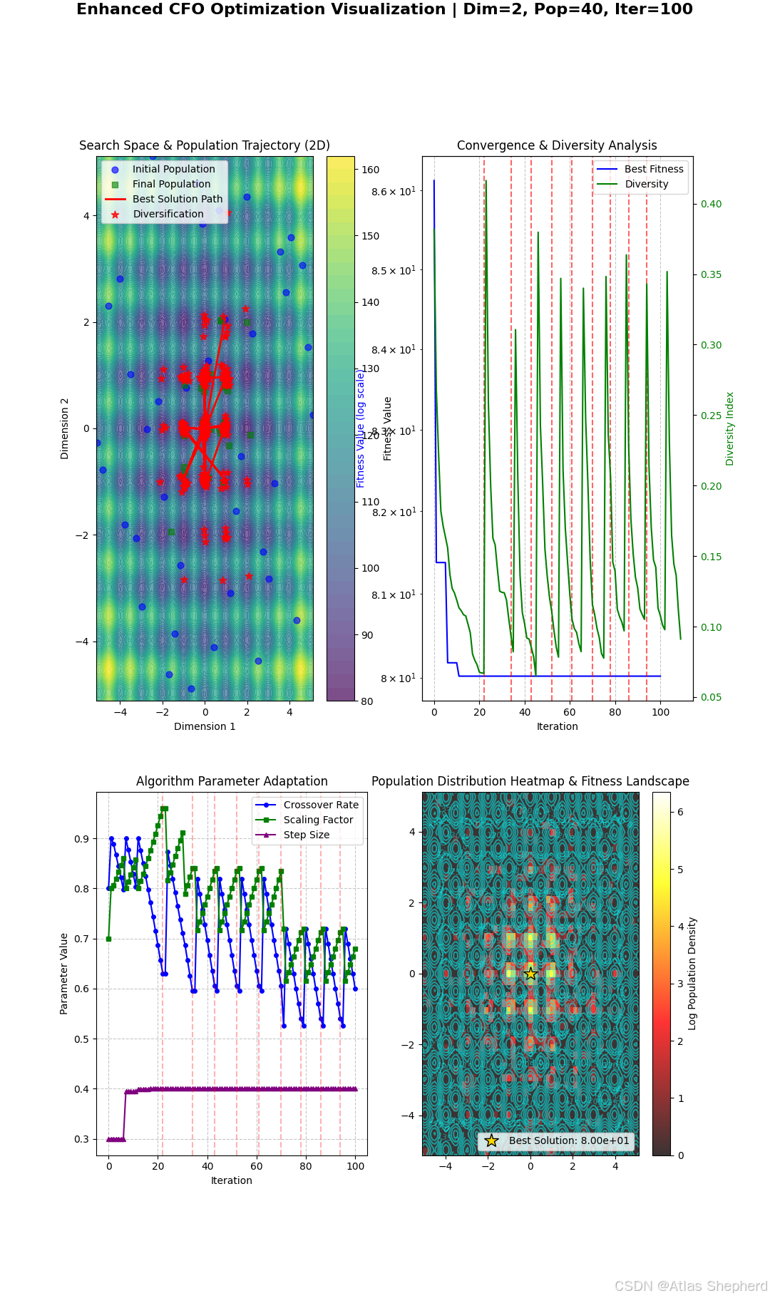
from sklearn.decomposition import PCAwarnings.filterwarnings("ignore")class EnhancedCFO:def __init__(self, objective_func, dim=10, pop_size=30, max_iter=200, lb=-10, ub=10):"""增强版冬虫夏草优化算法 - 针对后期停滞问题优化主要改进:1. 强化的停滞检测机制 - 加入适应度改善率和多样性指标2. 增强的多样化策略 - 多样化时引入方向性搜索3. 精英种群协作机制 - 防止局部最优4. 自适应参数调整优化 - 更平滑的参数变化"""self.obj_func = objective_funcself.dim = dimself.pop_size = pop_sizeself.max_iter = max_iterself.lb = lbself.ub = ubself.range = ub - lb# 算法参数self.p = 0.6  # 精英寄生概率self.diversity_threshold = 0.15  # 多样性阈值初始值# 初始化种群self.positions = self.latin_hypercube_init()self.fitness = np.array([objective_func(x) for x in self.positions])# 初始化最优解min_idx = np.argmin(self.fitness)self.best_pos = self.positions[min_idx].copy()self.best_fit = self.fitness[min_idx]self.second_best = self.best_pos.copy()self.second_fit = self.best_fitself.best_history = [self.best_fit]  # 存储历史最优值# 记录优化过程self.convergence_curve = [self.best_fit]self.execution_time = 0self.stagnation_count = 0self.stagnation_threshold = 25  # 初始停滞阈值self.diversity_history = [self.calculate_diversity()]self.improvement_rate = []  # 记录改进率历史# 自适应参数self.crossover_rate = 0.8self.scaling_factor = 0.7self.adaptive_step_size = 0.3# 优化阶段标志self.phase_shift = 0self.diversify_count = 0self.last_improvement = 0self.runtime_start = time.time()# 新增可视化数据记录self.pop_history = [self.positions.copy()]  # 记录每代种群位置self.iteration_markers = []  # 记录关键迭代点self.pca_model = None  # PCA模型用于高维可视化# 修复缺失的属性初始化self.adaptive_step_size = 0.3self.crossover_rate = 0.8self.scaling_factor = 0.7# 修复参数历史记录初始化self.adaptive_history = {'crossover_rate': [self.crossover_rate],'scaling_factor': [self.scaling_factor],'step_size': [self.adaptive_step_size]}def latin_hypercube_init(self):"""改进的拉丁超立方抽样初始化 - 增强边界多样性"""samples = np.zeros((self.pop_size, self.dim))for i in range(self.dim):segment_size = (self.ub - self.lb) / self.pop_sizestart = self.lb + segment_size * np.random.rand()samples[:, i] = np.linspace(start, self.ub, self.pop_size)np.random.shuffle(samples[:, i])return samplesdef calculate_diversity(self):"""计算种群多样性指数 - 使用平均成对距离"""distances = pdist(self.positions, 'euclidean')return np.mean(distances) / (self.range * np.sqrt(self.dim))def update_best(self, t):"""更新全局最优解并检测停滞状态 - 增强停滞检测"""min_idx = np.argmin(self.fitness)current_best = self.fitness[min_idx]# 基于历史变化的动态容差if len(self.best_history) > 5:best_range = max(1e-10, abs(max(self.best_history[-5:]) - min(self.best_history[-5:])))tolerance = min(best_range * 0.1, abs(self.best_fit) * 5e-3)else:tolerance = max(1e-10, abs(self.best_fit) * (1e-3 + 1e-4 * (t / self.max_iter)))improvement = self.best_fit - current_best# 计算改进率（相对改进量）if improvement > tolerance:if self.best_fit != 0:rate = improvement / abs(self.best_fit)else:rate = improvementself.improvement_rate.append(rate)self.second_best = self.best_pos.copy()self.second_fit = self.best_fitself.best_fit = current_bestself.best_pos = self.positions[min_idx].copy()self.stagnation_count = 0self.last_improvement = tself.best_history.append(self.best_fit)return Trueelse:self.stagnation_count += 1self.improvement_rate.append(0)  # 没有改进return Falsedef adaptive_params(self, t):"""动态调整算法参数 - 平滑过渡"""progress = t / self.max_iter# 基于改进率的自适应参数if len(self.improvement_rate) > 10:recent_improvement = np.mean(self.improvement_rate[-10:])step_size = max(0.1, min(0.5, 0.4 * np.exp(-10 * recent_improvement)))self.adaptive_step_size = step_sizeelse:step_size = self.adaptive_step_size# 基于种群多样性的参数调整diversity = self.diversity_history[-1]self.diversity_threshold = max(0.05, 0.2 * np.exp(-5 * diversity))# 三阶段策略if progress < 0.3:self.phase_shift = 1self.stagnation_threshold = max(20, 25 * (1 - progress))cr = 0.9sf = 0.8elif progress < 0.7:self.phase_shift = 2self.stagnation_threshold = max(25, 30 * (1 - progress))cr = 0.85sf = 0.7else:self.phase_shift = 3self.stagnation_threshold = max(15, 20 * (1 - progress))  # 降低后期阈值cr = 0.75sf = 0.6# 基于停滞计数的参数调整stagnation_factor = min(1.0, self.stagnation_count / self.stagnation_threshold)cr *= 1 - stagnation_factor * 0.3sf *= 1 + stagnation_factor * 0.2  # 增加变异强度self.crossover_rate = crself.scaling_factor = sf# 记录参数历史self.adaptive_history['crossover_rate'].append(cr)self.adaptive_history['scaling_factor'].append(sf)self.adaptive_history['step_size'].append(self.adaptive_step_size)def hybrid_exploration(self, t):"""增强混合探索策略 - 引入方向导数"""improved = Falsefor i in range(self.pop_size):if np.random.rand() < 0.7:# 基于方向的探索direction = self.best_pos - self.positions[i]direction /= np.linalg.norm(direction) + 1e-10# 自适应步长step_size = self.adaptive_step_size * (1.0 + np.random.randn() * 0.5)step_vector = step_size * direction + np.random.randn(self.dim) * 0.3new_position = np.clip(self.positions[i] + step_vector, self.lb, self.ub)else:# 差分进化 - 引入最优向量idxs = np.random.choice(self.pop_size, 3, replace=False)r1, r2, r3 = self.positions[idxs]if np.random.rand() < 0.5:  # 50%概率使用最优向量best_weight = np.random.rand() * 0.7mutation = (r1 + self.best_pos) * best_weight + self.scaling_factor * (r2 - r3)else:mutation = r1 + self.scaling_factor * (r2 - r3)cross_points = np.random.rand(self.dim) < self.crossover_rateif not np.any(cross_points):cross_points[np.random.randint(self.dim)] = Truenew_position = np.where(cross_points, mutation, self.positions[i])new_position = np.clip(new_position, self.lb, self.ub)# 评估并更新new_fitness = self.obj_func(new_position)if new_fitness < self.fitness[i]:self.positions[i] = new_positionself.fitness[i] = new_fitnessif new_fitness < self.best_fit:improved = True# 更新全局最优improved = self.update_best(t) or improvedreturn improveddef elite_mutation(self, intensity=1.0):"""精英突变算子 - 自适应突变强度"""elite_count = max(3, int(self.pop_size * 0.15))elite_indices = np.argsort(self.fitness)[:elite_count]for idx in elite_indices:# 基于停滞计数的自适应突变强度mutation_intensity = (self.ub - self.lb) * 0.08 * (intensity + self.stagnation_count / self.stagnation_threshold)mutation = mutation_intensity * np.random.randn(self.dim)new_position = np.clip(self.positions[idx] + mutation, self.lb, self.ub)new_fitness = self.obj_func(new_position)if new_fitness < self.fitness[idx]:self.positions[idx] = new_positionself.fitness[idx] = new_fitnessif new_fitness < self.best_fit:self.update_best(self.last_improvement)# 精英协作机制 - 前10%精英交换信息for i in range(1, len(elite_indices)):# 精英个体间交换部分维度信息swap_dims = np.random.choice(self.dim, size=max(1, int(self.dim * 0.3)), replace=False)for dim_idx in swap_dims:temp = self.positions[elite_indices[i - 1], dim_idx]self.positions[elite_indices[i - 1], dim_idx] = self.positions[elite_indices[i], dim_idx]self.positions[elite_indices[i], dim_idx] = temp# 重新评估适应度self.fitness[elite_indices[i - 1]] = self.obj_func(self.positions[elite_indices[i - 1]])self.fitness[elite_indices[i]] = self.obj_func(self.positions[elite_indices[i]])def spiral_rising(self, t):"""增强螺旋上升算子 - 非线性适应性螺旋"""improved = False# 基于进化阶段的自适应螺旋参数a = 0.4 - 0.3 * (t / self.max_iter)b = 0.5 + 1.0 * (t / self.max_iter)# 三引导源（动态权重）weights = np.random.dirichlet(np.ones(3), 1)[0]target = weights[0] * self.best_pos + weights[1] * self.second_best + weights[2] * self.positions[np.random.randint(self.pop_size)]for i in range(self.pop_size):# 自适应螺旋参数r_val = a * np.exp(b * 2 * np.pi * np.random.rand())# 方向向量direction = target - self.positions[i]direction /= np.linalg.norm(direction) + 1e-10# 螺旋运动加上随机扰动random_component = 0.1 * np.random.randn(self.dim)new_position = self.positions[i] + r_val * direction + random_componentnew_position = np.clip(new_position, self.lb, self.ub)# 评估并更新new_fitness = self.obj_func(new_position)if new_fitness < self.fitness[i]:self.positions[i] = new_positionself.fitness[i] = new_fitnessif new_fitness < self.best_fit:improved = True# 更新全局最优improved = self.update_best(t) or improvedreturn improveddef cooperative_parasitism(self, t):"""协同寄生机制 - 多宿主策略"""improved = Falsefitness_order = np.argsort(self.fitness)elite_count = max(5, int(self.pop_size * 0.3))elite_pool = fitness_order[:elite_count]ordinary_pool = fitness_order[elite_count:]for i in range(self.pop_size):# 精英宿主概率自适应调整elite_prob = max(0.4, min(0.8, self.p * (1 - t / self.max_iter)))# 多宿主策略（随机选择1-3个宿主）host_count = np.random.randint(1, 4)displacement = np.zeros(self.dim)for _ in range(host_count):if np.random.rand() < elite_prob and elite_pool.size > 0:host_idx = elite_pool[np.random.randint(len(elite_pool))]else:host_idx = ordinary_pool[np.random.randint(len(ordinary_pool))] if ordinary_pool.size > 0 else i# 自适应步长控制step_size = self.adaptive_step_size * (1.0 + np.random.randn() * 0.3)displacement += step_size * (self.positions[host_idx] - self.positions[i])displacement /= host_count  # 平均位移new_position = np.clip(self.positions[i] + displacement, self.lb, self.ub)# 评估并更新new_fitness = self.obj_func(new_position)if new_fitness < self.fitness[i]:self.positions[i] = new_positionself.fitness[i] = new_fitnessif new_fitness < self.best_fit:improved = True# 更新全局最优improved = self.update_best(t) or improvedreturn improveddef diversify_population(self, t):"""增强多样化策略 - 方向性多样化"""self.diversify_count += 1elite_count = max(5, int(self.pop_size * 0.25))elite_indices = np.argsort(self.fitness)[:elite_count]elite_positions = self.positions[elite_indices].copy()# 方向性多样化mean_position = np.mean(self.positions, axis=0)for i in range(self.pop_size):if i not in elite_indices:# 选择一个精英作为方向参考elite_ref = elite_positions[np.random.randint(elite_count)]# 多样化方向：远离种群中心或向精英方向探索if np.random.rand() < 0.7:# 远离种群中心direction = self.positions[i] - mean_positionelse:# 向精英方向探索direction = elite_ref - self.positions[i]direction /= np.linalg.norm(direction) + 1e-10# 自适应多样化步长mutate_factor = 0.4 + 0.3 * self.stagnation_count / self.stagnation_thresholdmutation = mutate_factor * (self.ub - self.lb) * direction * np.random.randn()self.positions[i] = np.clip(self.positions[i] + mutation, self.lb, self.ub)self.fitness[i] = self.obj_func(self.positions[i])# 更新精英位置 - 小幅扰动for i, idx in enumerate(elite_indices):mutation = 0.1 * (self.ub - self.lb) * np.random.randn(self.dim)elite_positions[i] = np.clip(elite_positions[i] + mutation, self.lb, self.ub)self.positions[idx] = elite_positions[i]self.fitness[idx] = self.obj_func(elite_positions[i])# 更新全局最优min_idx = np.argmin(self.fitness)if self.fitness[min_idx] < self.best_fit:self.best_pos = self.positions[min_idx].copy()self.best_fit = self.fitness[min_idx]self.best_history.append(self.best_fit)self.stagnation_count = 0diversity = self.calculate_diversity()self.diversity_history.append(diversity)self.iteration_markers.append(("diversify", t, self.best_fit))def optimize(self):"""主优化流程 - 增强停滞检测与处理"""print(f"Starting Enhanced CFO v2 | DIM: {self.dim} | POP: {self.pop_size}")print("Iter    Best Fitness    Diversity    Stag    ImpRate")print("----------------------------------------------------")self.runtime_start = time.time()for t in range(self.max_iter):self.adaptive_params(t)# 基于改进率的停滞检测stagnation_condition = Falseif len(self.improvement_rate) > 5:# 计算最近n次迭代的平均改进率recent_improvement = np.mean(self.improvement_rate[-5:])# 检测改进停滞：连续5次平均改进率小于阈值stagnation_condition = (recent_improvement < 1e-5 andself.stagnation_count > self.stagnation_threshold)# 执行多样化if stagnation_condition:self.diversify_population(t)# 多样化后进行一次精英突变增强self.elite_mutation(intensity=1.5)# 重置无重大改进的计数器current_improvement = False# 阶段优化策略if self.phase_shift == 1:current_improvement = self.hybrid_exploration(t) or current_improvementcurrent_improvement = self.cooperative_parasitism(t) or current_improvementelif self.phase_shift == 2:current_improvement = self.hybrid_exploration(t) or current_improvementcurrent_improvement = self.cooperative_parasitism(t) or current_improvementcurrent_improvement = self.spiral_rising(t) or current_improvementelse:current_improvement = self.spiral_rising(t) or current_improvementcurrent_improvement = self.cooperative_parasitism(t) or current_improvementself.elite_mutation()  # 后期增强精英突变# 记录当前种群状态self.pop_history.append(self.positions.copy())diversity = self.calculate_diversity()self.diversity_history.append(diversity)# 记录收敛曲线self.convergence_curve.append(self.best_fit)# 进度报告if t % 20 == 0 or t == self.max_iter - 1 or current_improvement:imp_rate = self.improvement_rate[-1] if self.improvement_rate else 0print(f"{t:4d}    {self.best_fit:.6e}    {diversity:.4f}    {self.stagnation_count:2d}    {imp_rate:.3e}")# 完成优化self.execution_time = time.time() - self.runtime_startprint("\nOptimization Completed!")print(f"Execution time: {self.execution_time:.2f} seconds")print(f"Best Fitness: {self.best_fit:.8e}")print(f"Diversifications: {self.diversify_count}")# 训练PCA模型用于高维可视化if self.dim > 3:all_positions = np.vstack(self.pop_history)self.pca_model = PCA(n_components=2)self.pca_model.fit(all_positions)return self.best_pos, self.best_fit, self.convergence_curvedef enhanced_visualization(self, save_path=None):"""增强版可视化：多维分析+动画+热力图"""fig = plt.figure(figsize=(18, 12), constrained_layout=True)fig.suptitle(f'Enhanced CFO Optimization Visualization | Dim={self.dim}, Pop={self.pop_size}, Iter={self.max_iter}',fontsize=16, fontweight='bold')gs = gridspec.GridSpec(2, 2, figure=fig, width_ratios=[1, 1], height_ratios=[1.5, 1])# 1. 搜索空间可视化面板ax1 = fig.add_subplot(gs[0, 0], projection='3d' if self.dim >= 3 else None)# 为低维问题创建搜索网格if self.dim == 2:x = np.linspace(self.lb, self.ub, 100)y = np.linspace(self.lb, self.ub, 100)X, Y = np.meshgrid(x, y)Z = np.zeros_like(X)for i in range(100):for j in range(100):Z[i, j] = self.obj_func(np.array([X[i, j], Y[i, j]]))# 绘制等高线contour = ax1.contourf(X, Y, Z, levels=50, cmap='viridis', alpha=0.7)fig.colorbar(contour, ax=ax1, label='Fitness Value')# 绘制初始和最终种群ax1.scatter(self.pop_history[0][:, 0], self.pop_history[0][:, 1],c='blue', s=40, marker='o', alpha=0.6, label='Initial Population')ax1.scatter(self.pop_history[-1][:, 0], self.pop_history[-1][:, 1],c='green', s=40, marker='s', alpha=0.6, label='Final Population')# 绘制最佳解轨迹best_traj = [pop[np.argmin([self.obj_func(x) for x in pop])] for pop in self.pop_history]best_traj = np.array(best_traj)ax1.plot(best_traj[:, 0], best_traj[:, 1], 'r-', linewidth=2, label='Best Solution Path')# 标记多样化位置for marker in self.iteration_markers:iter_idx = marker[1]if len(self.pop_history) > iter_idx:diver_pop = self.pop_history[iter_idx]ax1.scatter(diver_pop[:, 0], diver_pop[:, 1], c='red', s=60,marker='*', alpha=0.8,label='Diversification' if marker == self.iteration_markers[0] else '')ax1.set_title('Search Space & Population Trajectory (2D)')ax1.set_xlabel('Dimension 1')ax1.set_ylabel('Dimension 2')ax1.legend()elif self.dim >= 3:if self.dim > 3:# 绘制PCA投影pca_history = [self.pca_model.transform(pop) for pop in self.pop_history]# 绘制所有种群的PCA投影colors = plt.cm.jet(np.linspace(0, 1, len(pca_history)))for i, proj in enumerate(pca_history):ax1.scatter(proj[:, 0], proj[:, 1], color=colors[i], s=20,alpha=0.2 + 0.8 * i / len(pca_history))# 绘制最佳解的轨迹best_proj_history = []for i, pop in enumerate(self.pop_history):best_idx = np.argmin([self.obj_func(x) for x in pop])best_proj_history.append(pca_history[i][best_idx])best_proj = np.array(best_proj_history)ax1.plot(best_proj[:, 0], best_proj[:, 1], 'r-', linewidth=2, alpha=0.7)ax1.scatter(best_proj[-1, 0], best_proj[-1, 1], s=100, c='gold',marker='*', edgecolor='k', label='Best Solution')# 标记多样化位置for marker in self.iteration_markers:iter_idx = marker[1]if len(pca_history) > iter_idx:ax1.scatter(pca_history[iter_idx][:, 0], pca_history[iter_idx][:, 1],s=80, facecolors='none', edgecolors='r',linewidth=1.5,label='Diversification' if marker == self.iteration_markers[0] else '')ax1.set_xlabel('Principal Component 1')ax1.set_ylabel('Principal Component 2')ax1.set_title('Population Dynamics Projection (PCA)')# 添加颜色条表示迭代进度sm = plt.cm.ScalarMappable(cmap=plt.cm.jet, norm=plt.Normalize(vmin=0, vmax=self.max_iter))sm.set_array([])cbar = fig.colorbar(sm, ax=ax1, label='Iteration')else:# 3D空间的轨迹可视化ax1 = fig.add_subplot(gs[0, 0], projection='3d')# 绘制初始和最终种群ax1.scatter(self.pop_history[0][:, 0], self.pop_history[0][:, 1],self.pop_history[0][:, 2], c='blue', s=30, label='Initial Population')ax1.scatter(self.pop_history[-1][:, 0], self.pop_history[-1][:, 1],self.pop_history[-1][:, 2], c='green', s=50, marker='s', label='Final Population')# 绘制最佳解轨迹best_traj = [pop[np.argmin([self.obj_func(x) for x in pop])] for pop in self.pop_history]best_traj = np.array(best_traj)ax1.plot(best_traj[:, 0], best_traj[:, 1], best_traj[:, 2],'r-', linewidth=2, label='Best Solution Path')# 标记多样化位置for marker in self.iteration_markers:iter_idx = marker[1]if len(self.pop_history) > iter_idx:diver_pop = self.pop_history[iter_idx]ax1.scatter(diver_pop[:, 0], diver_pop[:, 1], diver_pop[:, 2],c='red', s=60, marker='*', alpha=0.8,label='Diversification' if marker == self.iteration_markers[0] else '')ax1.set_title('Population Trajectory in 3D Search Space')ax1.set_xlabel('Dimension 1')ax1.set_ylabel('Dimension 2')ax1.set_zlabel('Dimension 3')ax1.legend()# 2. 收敛分析面板ax2 = fig.add_subplot(gs[0, 1])# 绘制收敛曲线convergence_line = ax2.semilogy(self.convergence_curve, 'b-', linewidth=1.5, label='Best Fitness')[0]ax2.set_xlabel('Iteration')ax2.set_ylabel('Fitness Value (log scale)', color='b')ax2.tick_params(axis='y', labelcolor='b')ax2.grid(True, linestyle='--', alpha=0.7)# 添加多样性曲线ax3 = ax2.twinx()diversity_line = ax3.plot(self.diversity_history, 'g-', linewidth=1.5, label='Diversity')[0]ax3.set_ylabel('Diversity Index', color='g')ax3.tick_params(axis='y', labelcolor='g')# 标记多样化操作for marker in self.iteration_markers:t, fitness = marker[1], marker[2]ax2.axvline(x=t, color='r', linestyle='--', alpha=0.6)ax2.text(t, self.convergence_curve[t] * 10, 'Diversification',rotation=90, fontsize=9, ha='right', va='bottom')# 添加图例lines = [convergence_line, diversity_line]ax2.legend(lines, [l.get_label() for l in lines], loc='upper right')ax2.set_title('Convergence & Diversity Analysis')# 3. 参数动态变化面板ax4 = fig.add_subplot(gs[1, 0])# 修复：确保所有参数历史长度一致min_length = min(len(self.adaptive_history['crossover_rate']),len(self.adaptive_history['scaling_factor']),len(self.adaptive_history['step_size']))# 提取参数历史iterations = np.arange(min_length)# 绘制参数变化曲线ax4.plot(iterations, self.adaptive_history['crossover_rate'][:min_length],'o-', markersize=4, linewidth=1.5, color='blue', label='Crossover Rate')ax4.plot(iterations, self.adaptive_history['scaling_factor'][:min_length],'s-', markersize=4, linewidth=1.5, color='green', label='Scaling Factor')ax4.plot(iterations, self.adaptive_history['step_size'][:min_length],'^-', markersize=4, linewidth=1.5, color='purple', label='Step Size')ax4.set_xlabel('Iteration')ax4.set_ylabel('Parameter Value')ax4.legend()ax4.grid(True, linestyle='--', alpha=0.7)ax4.set_title('Algorithm Parameter Adaptation')# 标记参数变化点for marker in self.iteration_markers:if marker[1] < min_length:ax4.axvline(x=marker[1], color='r', linestyle='--', alpha=0.3)# 4. 种群密度与位置热图面板ax5 = fig.add_subplot(gs[1, 1])if self.dim == 2:# 创建密度网格x_bins = np.linspace(self.lb, self.ub, 50)y_bins = np.linspace(self.lb, self.ub, 50)density = np.zeros((len(y_bins) - 1, len(x_bins) - 1))# 统计所有迭代中的个体位置for pop in self.pop_history:for ind in pop:x_idx = np.digitize(ind[0], x_bins) - 1y_idx = np.digitize(ind[1], y_bins) - 1if 0 <= x_idx < density.shape[1] and 0 <= y_idx < density.shape[0]:density[y_idx, x_idx] += 1# 应用对数缩放density = np.log1p(density)# 绘制热力图im = ax5.imshow(density, cmap='hot', origin='lower',extent=[self.lb, self.ub, self.lb, self.ub],aspect='auto', alpha=0.8)# 添加等高线x = np.linspace(self.lb, self.ub, 100)y = np.linspace(self.lb, self.ub, 100)X, Y = np.meshgrid(x, y)Z = np.zeros_like(X)for i in range(100):for j in range(100):Z[i, j] = self.obj_func(np.array([X[i, j], Y[i, j]]))contours = ax5.contour(X, Y, Z, levels=15, colors='cyan', alpha=0.5)ax5.clabel(contours, inline=True, fontsize=8, fmt='%1.1f')# 绘制最佳解位置ax5.plot(self.best_pos[0], self.best_pos[1], '*', markersize=15,markeredgecolor='black', markerfacecolor='gold',label=f'Best Solution: {self.best_fit:.2e}')# 添加颜色条fig.colorbar(im, ax=ax5, label='Log Population Density')ax5.set_title('Population Distribution Heatmap & Fitness Landscape')ax5.legend()else:ax5.text(0.5, 0.5, 'Population heatmap only available for 2D problems',ha='center', va='center', fontsize=12)ax5.set_title('Population Heatmap Not Available for High Dimensions')# 保存结果if save_path:plt.savefig(save_path, dpi=150, bbox_inches='tight')print(f"Enhanced visualization saved to {save_path}")plt.show()# 如果维度为2，创建进化过程动画if self.dim == 2 and len(self.pop_history) > 1:print("\nGenerating optimization animation...")self.create_animation()return figdef create_animation(self, filename='cfo_animation.gif'):"""创建优化过程动画 (仅适用于2D问题)"""if self.dim != 2:print("Animation only available for 2D problems")return# 创建网格用于可视化x = np.linspace(self.lb, self.ub, 100)y = np.linspace(self.lb, self.ub, 100)X, Y = np.meshgrid(x, y)Z = np.zeros_like(X)for i in range(100):for j in range(100):Z[i, j] = self.obj_func(np.array([X[i, j], Y[i, j]]))# 减少帧数以加速动画step = max(1, len(self.pop_history) // 100)frames = range(0, len(self.pop_history), step)fig, ax = plt.subplots(figsize=(10, 8))contour = ax.contourf(X, Y, Z, levels=50, cmap='viridis', alpha=0.7)fig.colorbar(contour, ax=ax, label='Fitness Value')ax.set_xlim(self.lb, self.ub)ax.set_ylim(self.lb, self.ub)ax.set_xlabel('Dimension 1')ax.set_ylabel('Dimension 2')ax.set_title('Enhanced CFO Optimization Process')# 初始散点图scat = ax.scatter([], [], s=50, c='white', ec='black', alpha=0.8, zorder=3)best_point = ax.scatter([], [], s=100, marker='*', c='gold', ec='black', zorder=4)best_traj, = ax.plot([], [], 'r-', linewidth=1.5, zorder=2)best_positions = []iteration_text = ax.text(0.05, 0.95, '', transform=ax.transAxes,fontsize=12, bbox=dict(facecolor='white', alpha=0.8))fitness_text = ax.text(0.05, 0.90, '', transform=ax.transAxes,fontsize=10, bbox=dict(facecolor='white', alpha=0.8))# 动画更新函数def update(frame):ax.collections = [ax.collections[0]]  # 只保留背景pop = self.pop_history[frame]scat.set_offsets(pop)# 更新颜色表示适应度colors = np.array([self.obj_func(x) for x in pop])norm = mcolors.Normalize(vmin=colors.min(), vmax=colors.max())cmap = cm.plasmascat.set_color(cmap(norm(colors)))# 更新最佳解best_idx = np.argmin(colors)current_best = pop[best_idx]best_point.set_offsets([current_best])# 记录最佳解轨迹best_positions.append(current_best)if len(best_positions) > 1:best_traj.set_data(*zip(*best_positions))# 更新文本iteration_text.set_text(f'Iteration: {frame}/{len(self.pop_history) - 1}')fitness_text.set_text(f'Best Fitness: {colors.min():.4e}\nPopulation Diversity: {self.diversity_history[frame]:.4f}')return scat, best_point, best_traj, iteration_text, fitness_text# 创建动画ani = FuncAnimation(fig, update, frames=frames, interval=100, blit=True)# 保存动画print(f"Saving animation to {filename}...")ani.save(filename, writer='pillow', fps=10)print("Animation saved successfully!")plt.close(fig)return ani# 测试函数定义
def test_function(func_name, dim=10):"""测试函数工厂"""def sphere(x):return np.sum(x ** 2)def rastrigin(x):A = 10return A * dim + np.sum(x ** 2 - A * np.cos(2 * np.pi * x))def rosenbrock(x):return np.sum(100.0 * (x[1:] - x[:-1] ** 2.0) ** 2.0 + (1 - x[:-1]) ** 2.0)def ackley(x):a = 20b = 0.2c = 2 * np.pin = len(x)sum1 = np.sum(x ** 2)sum2 = np.sum(np.cos(c * x))term1 = -a * np.exp(-b * np.sqrt(sum1 / n))term2 = -np.exp(sum2 / n)return term1 + term2 + a + np.exp(1)def griewank(x):sum1 = np.sum(x ** 2) / 4000prod1 = np.prod(np.cos(x / np.sqrt(np.arange(1, len(x) + 1))))return sum1 - prod1 + 1def schwefel(x):return 418.9829 * dim - np.sum(x * np.sin(np.sqrt(np.abs(x))))func_map = {'sphere': sphere,'rastrigin': rastrigin,'rosenbrock': rosenbrock,'ackley': ackley,'griewank': griewank,'schwefel': schwefel}return func_map.get(func_name.lower(), sphere)def benchmark(test_funcs=None, dim=10, runs=5):"""基准测试套件"""if test_funcs is None:test_funcs = ['sphere', 'rastrigin', 'rosenbrock', 'ackley', 'griewank']results = {}for func_name in test_funcs:print(f"\n=== Benchmarking {func_name} function (Dim={dim}) ===")best_fitness = []exec_times = []for i in range(runs):print(f"\nRun {i + 1}/{runs}")optimizer = EnhancedCFO(objective_func=test_function(func_name, dim),dim=dim,pop_size=50,max_iter=300)_, fitness, _ = optimizer.optimize()best_fitness.append(fitness)exec_times.append(optimizer.execution_time)# 每次运行后调用增强可视化if dim in [2, 3]:optimizer.enhanced_visualization(save_path=f"{func_name}_result_{i + 1}.png")avg_fitness = np.mean(best_fitness)avg_time = np.mean(exec_times)std_fitness = np.std(best_fitness)results[func_name] = {'best_fitness': best_fitness,'average_fitness': avg_fitness,'std_fitness': std_fitness,'execution_times': exec_times,'average_time': avg_time}print(f"\n{func_name} Results:")print(f"  Average Fitness: {avg_fitness:.6e}")print(f"  Fitness Std Dev: {std_fitness:.6e}")print(f"  Average Execution Time: {avg_time:.2f}s")# 打印总结报告print("\n=== Benchmark Summary ===")for func, res in results.items():print(f"{func:15} | Best: {min(res['best_fitness']):.2e} | Avg: {res['average_fitness']:.2e} | Std: {res['std_fitness']:.2e}")return resultsif __name__ == "__main__":# 单个函数优化示例（添加可视化）optimizer = EnhancedCFO(objective_func=test_function("rastrigin"),dim=2,  # 改为2维以启用完整可视化pop_size=40,max_iter=100,lb=-5.12,ub=5.12)best_solution, best_fitness, convergence = optimizer.optimize()optimizer.enhanced_visualization(save_path="enhanced_cfo_visualization.png")print("\n=== Solution Validation ===")print(f"Best Fitness: {best_fitness:.10f}")print("Best Solution Vector:")print(np.around(best_solution, 4))# 使用gif动画需要启用以下行# optimizer.create_animation()# 完整基准测试（可选）# benchmark(dim=2, runs=1)  # 二维测试以便可视化