Title
题目
Hierarchical Vision Transformers for prostate biopsy grading: Towardsbridging the generalization gap
用于前列腺活检分级的分层视觉 Transformer:迈向弥合泛化差距
01
文献速递介绍
前列腺癌是全球男性中第二常见的确诊癌症,也是第五大致命癌症。病理学家对前列腺活检样本进行分级,在确定前列腺癌的侵袭性方面起着关键作用,进而指导从主动监测到手术等一系列干预措施。随着前列腺癌患者数量不断增加,病理学家的工作压力日益增大,因此迫切需要借助计算方法辅助日常工作流程。 组织切片的数字化使得大规模数据集的可获得性不断提高,这为计算机视觉研究创造了机会,有助于通过深度学习算法为病理学家提供支持和辅助。深度学习彻底改变了计算机视觉的多个领域,在图像分类、目标检测和语义分割等任务中取得了前所未有的成功。十年前,卷积神经网络(CNNs)取得了重大进展(Krizhevsky 等人,2012),而近年来,诸如视觉Transformer(ViT)(Dosovitskiy 等人,2021)等基于注意力机制的模型进一步突破了性能极限。 然而,由于全切片图像(WSIs)尺寸极大,超出了传统深度学习硬件的内存容量,计算病理学面临着一系列独特的挑战。因此,人们提出了创新策略来克服这一内存瓶颈。一种主流方法是将这些庞大的图像分割成更小的补丁。这些补丁通常作为输入单元,其标签来自像素级注释(Ehteshami Bejnordi 等人,2017;Coudray 等人,2018)。但获取像素级注释既耗时又不切实际,尤其是在前列腺癌分级等复杂任务中,病理学家只能对他们能识别的部分进行注释。因此,近年来的研究探索了超越全监督的技术,重点关注更灵活的训练范式,如弱监督学习。 弱监督学习利用粗粒度(图像级)信息自动推断细粒度(补丁级)细节。多实例学习(MIL)近年来在多项计算病理学挑战中成为一种强大的弱监督方法,并展现出卓越的性能(Hou 等人,2015;Campanella 等人,2019)。通过仅使用切片级标签就能对全切片图像进行分析,它避开了对像素级注释的需求,为风险预测和基因突变检测等任务提供了便利(Schmauch 等人,2020;Garberis 等人,2022)。 尽管多实例学习取得了成功,但大多数多实例学习方法忽略了补丁之间的空间关系,从而错失了有价值的上下文信息。为解决这一局限,研究重点转向开发能够整合更广泛上下文的方法(Lerousseau 等人,2021;Pinckaers 等人,2021;Shao 等人,2021)。其中,分层视觉Transformer(H-ViTs)已成为一种很有前景的解决方案,在癌症亚型分类和生存预测方面取得了最先进的成果(Chen 等人,2022)。 基于这些考虑,我们在前列腺癌分级背景下对分层视觉Transformer进行了全面分析。我们的工作在该领域取得了多项关键进展,具体如下: 1. 我们发现,当在与训练数据来自同一中心的病例上进行测试时,分层视觉Transformer与最先进的前列腺癌分级算法性能相当,同时在更多样化的临床场景中表现出更强的泛化能力。 2. 我们证明了针对前列腺的特异性预训练相比更通用的多器官预训练具有优势。 3. 我们系统地比较了两种分层视觉Transformer变体,并就每种变体更适用的场景提供了具体指导。 4. 我们对序数分类的损失函数选择进行了深入分析,表明将前列腺癌分级视为回归任务具有优越性。 5. 我们通过引入一种创新方法来整合分层Transformer中的注意力分数(平衡与任务无关和与任务相关的贡献),增强了模型的可解释性。
Abatract
摘要
Practical deployment of Vision Transformers in computational pathology has largely been constrained by thesheer size of whole-slide images. Transformers faced a similar limitation when applied to long documents, andHierarchical Transformers were introduced to circumvent it. This work explores the capabilities of HierarchicalVision Transformers for prostate cancer grading in WSIs and presents a novel technique to combine attentionscores smartly across hierarchical transformers. Our best-performing model matches state-of-the-art algorithmswith a 0.916 quadratic kappa on the Prostate cANcer graDe Assessment (PANDA) test set. It exhibits superiorgeneralization capacities when evaluated in more diverse clinical settings, achieving a quadratic kappa of0.877, outperforming existing solutions. These results demonstrate our approach’s robustness and practicaapplicability, paving the way for its broader adoption in computational pathology and possibly other medicalimaging tasks.
在计算病理学中,视觉Transformer(Vision Transformers)的实际部署在很大程度上受到全切片图像(whole-slide images)庞大尺寸的限制。Transformer在处理长文档时也面临类似的局限,而分层Transformer(Hierarchical Transformers)的引入正是为了规避这一问题。 本研究探索了分层视觉Transformer(Hierarchical Vision Transformers)在全切片图像(WSIs)前列腺癌分级中的性能,并提出了一种跨分层Transformer智能融合注意力分数的新技术。我们性能最佳的模型在前列腺癌分级评估(PANDA)测试集上达到了0.916的加权kappa系数,与最先进算法持平。在更多样化的临床场景中评估时,该模型展现出更优的泛化能力,加权kappa系数达0.877,优于现有解决方案。这些结果证明了我们方法的稳健性和实际适用性,为其在计算病理学及其他医学影像任务中的更广泛应用奠定了基础。
Background
背景
Method
方法
3.1. Hierarchical vision transformer
The inherent hierarchical structure within whole-slide images spansacross various scales, from tiny cell-centric regions – (16,16) pixels at0.50 microns per pixels (mpp) – containing fine-grained information, allthe way up to the entire slide, which exhibits the overall intra-tumoralheterogeneity of the tissue microenvironment. Along this spectrum,(256,256) patches depict cell-to-cell interactions, while larger regions– (1024,1024) to (4096,4096) pixels – capture macro-scale interactionsbetween clusters of cells.
3.1. 分层视觉Transformer 全切片图像中固有的层级结构跨越多种尺度:从小型细胞中心区域——即0.50微米/像素(mpp)分辨率下的(16,16)像素区域,包含细粒度信息;到整个切片,呈现肿瘤内组织微环境的整体异质性。在这一尺度范围内,(256,256)像素的补丁可描述细胞间的相互作用,而更大的区域——(1024,1024)至(4096,4096)像素——则能捕捉细胞集群间的宏观相互作用。
Conclusion
结论
In summary, our study demonstrates the transformative potential ofHierarchical Vision Transformers in predicting prostate cancer gradesfrom biopsies. By leveraging the inherent hierarchical structure ofWSIs, H-ViTs efficiently capture context-aware representations, addressing several shortcomings of conventional patch-based methods.Our findings set new benchmarks in prostate cancer grading. Ourmodel outperforms existing solutions when tested on a dataset thatuniquely represents the full diversity of cases seen in clinical practice,effectively narrowing the generalization gap in prostate biopsy grading.This work provides new insights that deepen our understanding of themechanisms underlying H-ViTs’ effectiveness. Our results showcase therobustness and adaptability of this method in a new setting, pavingthe way for its broader adoption in computational pathology andpotentially other medical imaging tasks.
总之,本研究证实了分层视觉Transformer(Hierarchical Vision Transformers)在通过活检样本预测前列腺癌分级方面的变革性潜力。借助全切片图像(WSIs)固有的层级结构,H-ViTs能够高效捕捉具备上下文感知的表征,从而解决了传统基于补丁的方法存在的诸多缺陷。 我们的研究结果为前列腺癌分级设立了新的基准。在测试数据集(该数据集独特地涵盖了临床实践中所见的各种病例)上,我们的模型性能优于现有解决方案,有效缩小了前列腺活检分级中的泛化差距。 这项工作提供了新的见解,加深了我们对H-ViTs有效性背后机制的理解。研究结果展示了该方法在新场景中的稳健性和适应性,为其在计算病理学及可能的其他医学影像任务中的更广泛应用铺平了道路。
Results
结果
6.1. Self-supervised pretraining
Pretraining the patch-level Transformer for 50 epochs took 3 dayson 4 GeForce RTX 3080 Ti. Fig. 4 shows the area under the curve(AUC) for teacher and student networks on the downstream patch-levelclassification dataset over pretraining epochs. Results are averagedacross the 5 cross validation folds. Early stopping was not triggeredfor any of the 5 folds. Pretraining the region-level Transformer on(4096, 4096) regions on 1 GeForce RTX 3080 Ti. More details aboutcomputational characteristics can be found in Appendix J.Classification results with CE loss are summarized in Table 2 (GlobalH-ViT) and Table 3 (Local H-ViT). Additional results for other lossfunctions can be found in Appendix A (Global H-ViT) and AppendixB (Local H-ViT). Overall, across all region sizes, models pretrainedon the PANDA dataset consistently achieve higher macro-averagedperformance than those pretrained on TCGA. Performance gains aremore significant for Global H-ViT (+68% on average) than for LocalH-ViT (+14% on average). This roots back to a common limitationof patch-based MIL: the disconnection between feature extraction andfeature aggregation. There is no guarantee the features extracted during pretraining are relevant for the downstream classification task.Allowing gradients to flow through the region-level Transformer partlyovercomes this limitation: Local H-ViT has more amplitude than GlobalH-ViT to refine the TCGA-pretrained features so that they better fit theclassification task at hand.
6.1. 自监督预训练 在4块GeForce RTX 3080 Ti显卡上,对补丁级Transformer进行50个 epoch的预训练耗时3天。图4展示了在预训练过程中,教师网络和学生网络在下游补丁级分类数据集上的曲线下面积(AUC)变化。结果为5折交叉验证的平均值,早期停止机制在5个折中均未触发。在1块GeForce RTX 3080 Ti显卡上对(4096, 4096)区域的区域级Transformer进行预训练的计算特性详情见附录J。 采用交叉熵(CE)损失的分类结果汇总于表2(Global H-ViT)和表3(Local H-ViT)。其他损失函数的补充结果见附录A(Global H-ViT)和附录B(Local H-ViT)。总体而言,在所有区域大小下,基于PANDA数据集预训练的模型在宏观平均性能上均优于基于TCGA数据集预训练的模型。Global H-ViT的性能提升更为显著(平均+68%),而Local H-ViT的提升相对温和(平均+14%)。这源于基于补丁的多实例学习(MIL)的一个常见局限:特征提取与特征聚合之间的脱节——无法保证预训练阶段提取的特征与下游分类任务相关。 允许梯度通过区域级Transformer传播可部分克服这一局限:与Global H-ViT相比,Local H-ViT拥有更大的调整空间,能够优化TCGA预训练特征,使其更适配当前的分类任务。
Figure
图
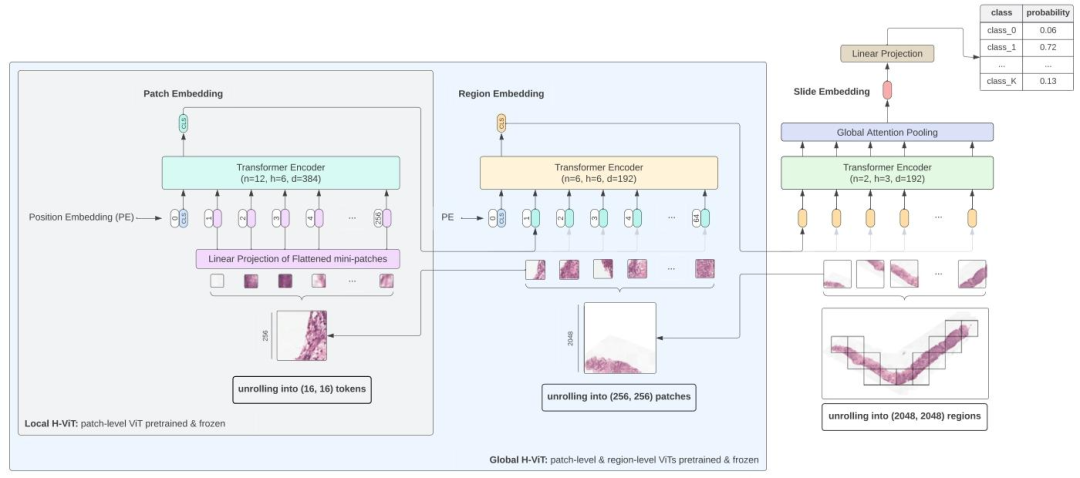
Fig. 1. Overview of our Hierarchical Vision Transformer for whole-slide image analysis. The model processes whole-slide images at multiple scales. Slides are unrolled into nonoverlapping 2048 × 2048 regions, which are further divided into 256 × 256 patches following a regular grid. First, a pretrained ViT-S/16 (referred to as the patch-level Transformer)embeds these patches into feature vectors. These patch-level features are then input to a second Transformer (referred to as the region-level Transformer), which aggregates theminto region-level embeddings. Finally, a third Transformer (referred to as the slide-level Transformer) pools the region-level embeddings into a slide-level representation, which isprojected to class logits for downstream task prediction. We experiment with two model variants: in Global H-ViT, both the patch-level and region-level Transformers are pretrainedand frozen, with only the slide-level Transformer undergoing weakly-supervised training; in Local H-ViT, only the patch-level Transformer is frozen, while both the region-leveland slide-level Transformers are trained using weak supervision
图1. 用于全切片图像分析的分层视觉Transformer概述 该模型以多尺度处理全切片图像:首先将切片展开为不重叠的2048×2048区域,这些区域再按规则网格进一步划分为256×256的补丁。第一步,预训练的ViT-S/16(称为补丁级Transformer)将这些补丁嵌入为特征向量;随后,这些补丁级特征被输入到第二个Transformer(称为区域级Transformer),聚合为区域级嵌入;最后,第三个Transformer(称为切片级Transformer)将区域级嵌入聚合为切片级表征,并映射为类别对数概率以用于下游任务预测。 我们对两种模型变体进行了实验: - 在Global H-ViT中,补丁级和区域级Transformer均经过预训练并固定参数,仅切片级Transformer进行弱监督训练; - 在Local H-ViT中,仅补丁级Transformer固定参数,区域级和切片级Transformer均通过弱监督进行训练。
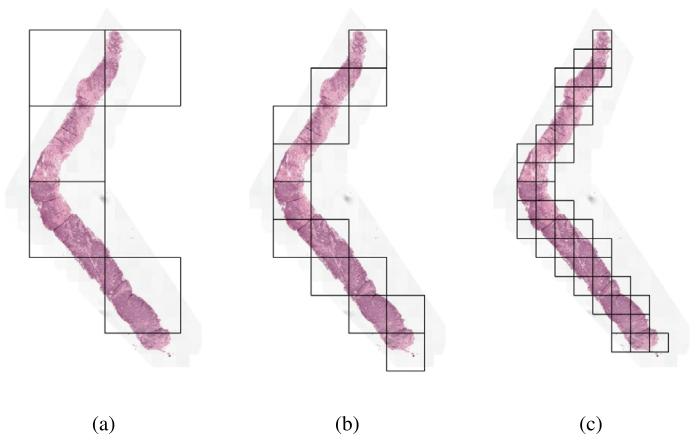
Fig. 2. Visualization of region extraction at 0.50 mpp for varying region sizes: (a)(4096, 4096) regions, (b) (2048, 2048) regions and (c) (1024, 1024) regions.
图 2. 0.50 微米 / 像素分辨率下不同区域大小的提取可视化(a) 4096×4096 像素区域(b) 2048×2048 像素区域(c) 1024×1024 像素区域
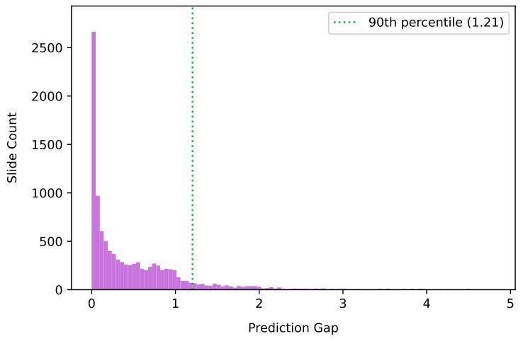
Fig. 3. Distribution of the prediction gap for PANDA development set
图3. PANDA开发集的预测差距分布
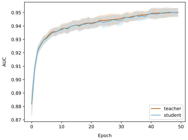
Fig. 4. Classification performance for teacher and student networks on the binaryclassification of prostate patches, used as downstream evaluation during pretraining.Lines represent the mean AUC across the 5 cross validation folds, with shaded areasindicating standard deviation.
4. 教师网络和学生网络在前列腺补丁二元分类任务上的分类性能(用于预训练期间的下游评估)线条代表 5 折交叉验证的平均 AUC(曲线下面积),阴影区域表示标准差。
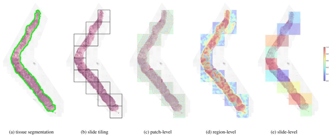
Fig. 5. Visualization of stitched attention heatmaps for each Transformer. We show the result of tissue segmentation (a) where tissue is delineated in green, and the result of slidetiling into non-overlapping (2048, 2048) regions as 0.50 mpp, keeping only regions with 10% tissue or more. For each of the three Transformers, we overlay the correspondingattention scores assigned to each element of the input sequence: (16, 16) tokens for the patch-level Transformer, (256, 256) patches for the region-level Transformer, and (2048,regions for the slide-level Transformer.
图 5. 各 Transformer 的拼接注意力热图可视化我们展示了组织分割结果 (a)(绿色勾勒出组织区域),以及将切片划分为 0.50 微米 / 像素分辨率下非重叠的 2048×2048 区域的结果(仅保留组织占比≥10% 的区域)。对于三个 Transformer,我们分别叠加了为输入序列各元素分配的注意力分数:补丁级 Transformer 对应(16,16)像素令牌,区域级 Transformer 对应(256,256)像素补丁,切片级 Transformer 对应(2048,2048)像素区域。
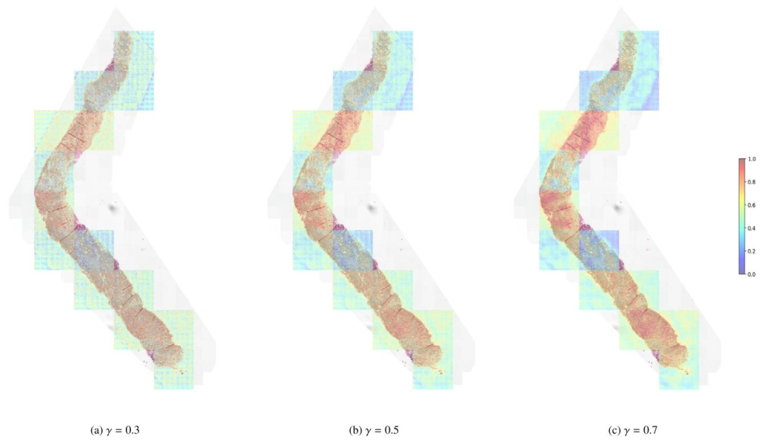
Fig. 6. Refined (2048,2048) factorized attention heatmaps of Local H-ViT for varying values of parameter 𝛾. In the context of prostate cancer grading, the relevant signal isfound within the tissue architecture, spanning intermediate to large scales. Since the patch-level Transformer primarily captures cell-level features, we recommend using 𝛾 > 0.5to emphasize coarser, task-specific features, rather than finer, task-agnostic details.
图 6. 不同参数*𝛾*值下 Local H-ViT 的精细化(2048,2048)因子注意力热图在前列腺癌分级场景中,相关信号存在于组织结构中,涵盖中等至较大尺度。由于补丁级 Transformer 主要捕捉细胞级特征,因此我们建议使用𝛾>0.5,以强调更粗略的、与任务相关的特征,而非更精细的、与任务无关的细节。
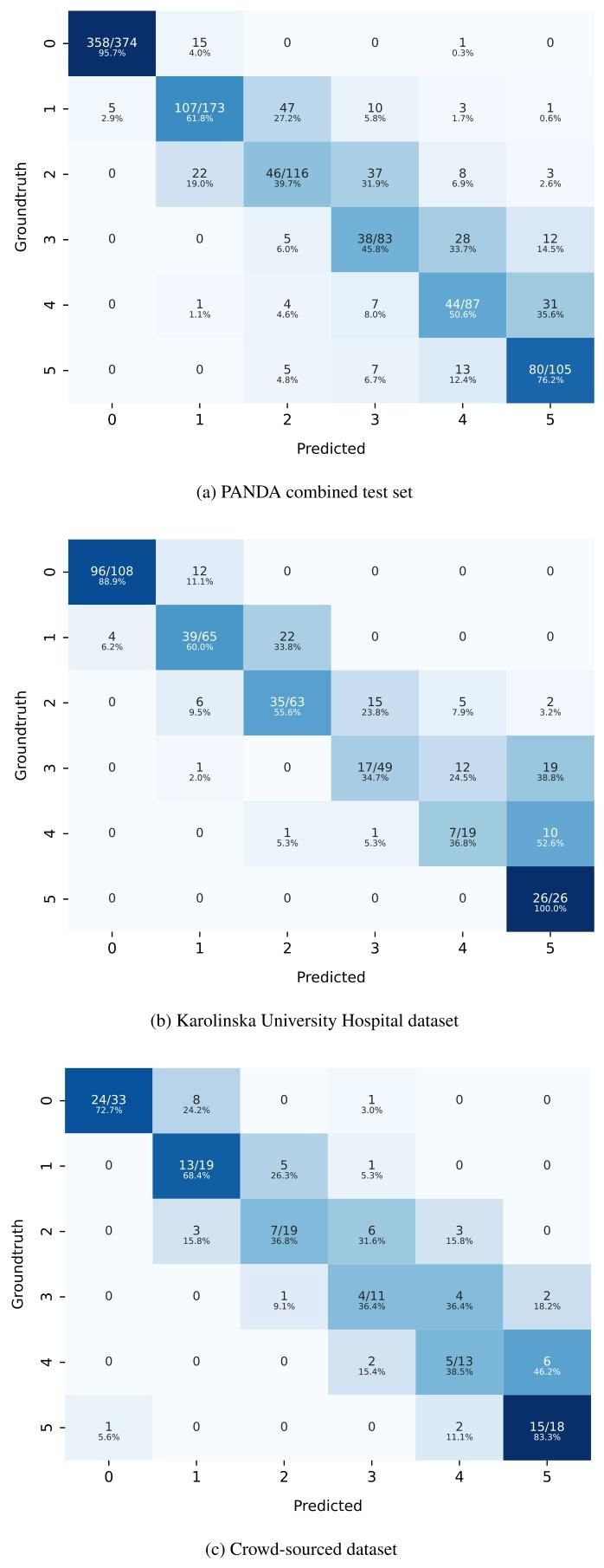
Fig. C.1. Confusion matrices of our best performing ensemble model on the 3 evaluation datasets.
图 C.1. 最佳集成模型在 3 个评估数据集上的混淆矩阵
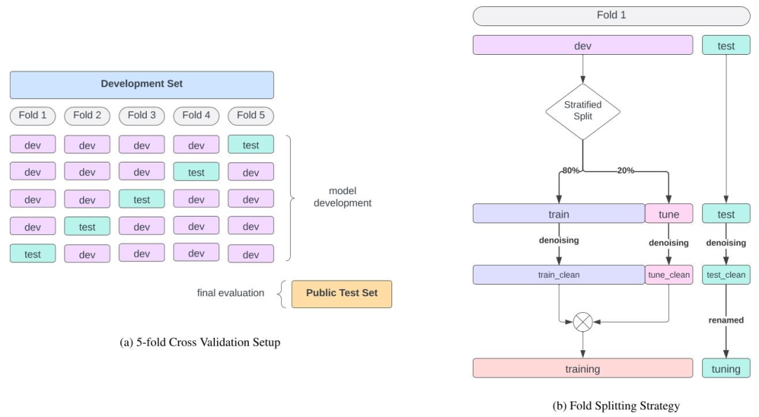
Fig. G.2. Overview of the 5-fold Cross Validation Splitting Strategy.
图 G.2. 5 折交叉验证分割策略概述
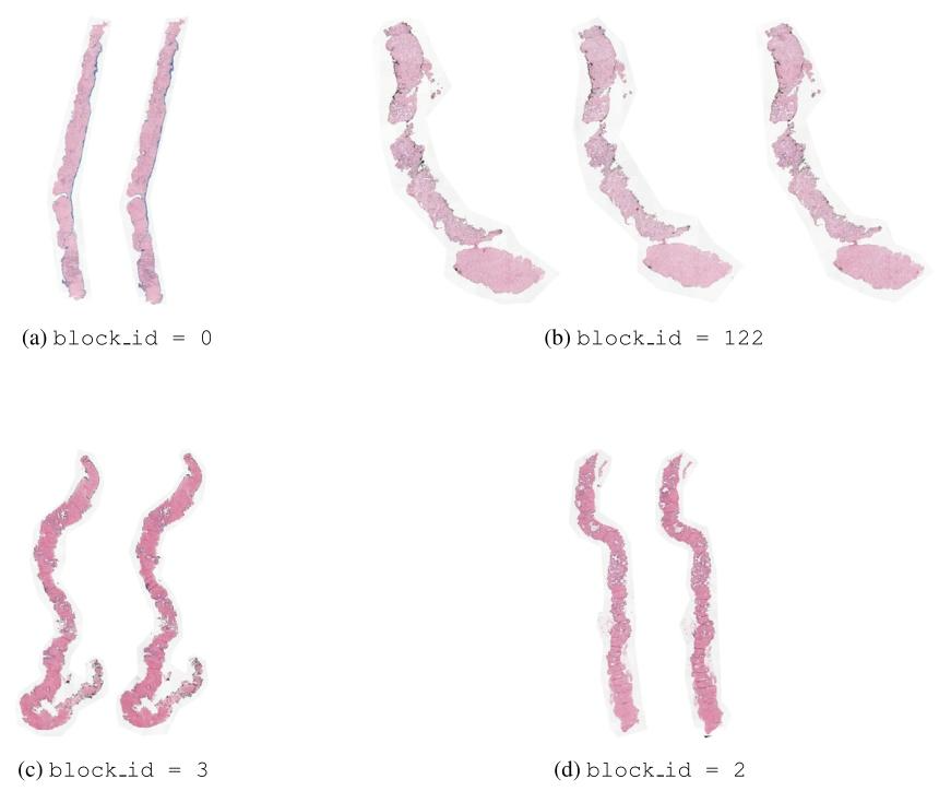
Fig. H.3. Visualization of four artificial blocks. (a), (c) and (d) show blocks with 2 slides. (b) shows a block with 3 slides.
图 H.3. 四个人工区块的可视化(a)、(c) 和 (d) 展示包含 2 张切片的区块,(b) 展示包含 3 张切片的区块。
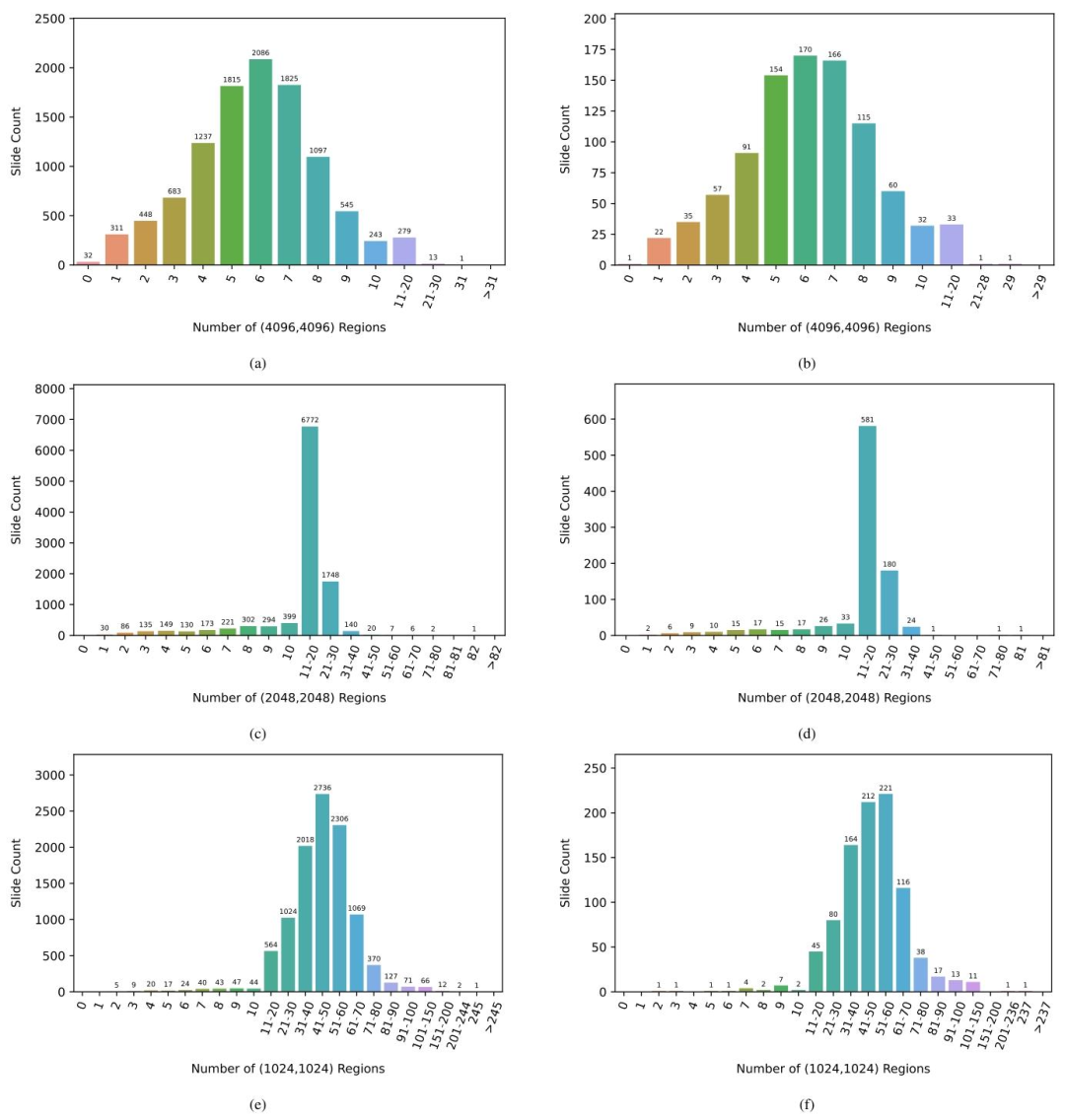
Fig. I.4. Distribution of the number of extracted regions for PANDA development set with (a) (4096, 4096) regions (c) (2048, 2048) regions (e) (1024, 1024) regions and forPANDA public test set with (b) (4096, 4096) regions (d) (2048, 2048) regions (f) (1024, 1024) regions.
图 I.4. PANDA 开发集和公开测试集中提取的区域数量分布开发集:(a) 4096×4096 像素区域的数量分布;(c) 2048×2048 像素区域的数量分布;(e) 1024×1024 像素区域的数量分布。公开测试集:(b) 4096×4096 像素区域的数量分布;(d) 2048×2048 像素区域的数量分布;(f) 1024×1024 像素区域的数量分布。
Table
表
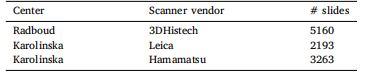
Table 1Scanner details, PANDA development set.
表 1 PANDA 开发集的扫描仪详情
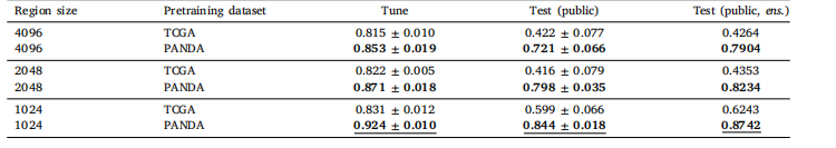
Table 2Classification performance of Global H-ViT for different pretraining configurations, obtained with cross-entropy loss. We report the mean andstandard deviation of the quadratic weighted kappa across the 5 cross-validation folds, along with the kappa score achieved by ensemblingpredictions from each fold.
表 2 不同预训练配置下 Global H-ViT 的分类性能(采用交叉熵损失)我们报告了 5 折交叉验证中加权 kappa 系数的均值和标准差,以及通过集成各折预测结果得到的 kappa 分数。
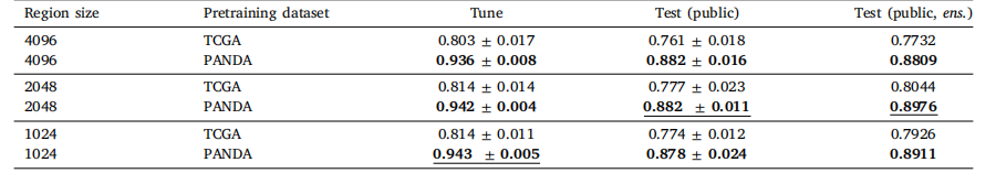
Table 3Classification performance of Local H-ViT for different pretraining configurations, obtained with cross-entropy loss. We report the mean andstandard deviation of the quadratic weighted kappa across the 5 cross-validation folds, along with the kappa score achieved by ensemblingpredictions from each fold.
表 3 不同预训练配置下 Local H-ViT 的分类性能(采用交叉熵损失)我们报告了 5 折交叉验证中加权 kappa 系数的均值和标准差,以及通过集成各折预测结果得到的 kappa 分数。
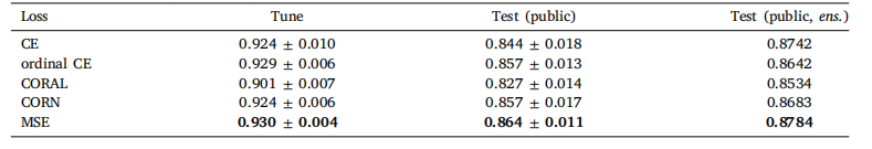
Table 4Classification performance of Global H-ViT for different loss functions, obtained with (1024, 1024) regions at 0.50 mpp. Wereport the mean and standard deviation of the quadratic weighted kappa across the 5 cross-validation folds, along with thekappa score achieved by ensembling predictions from each fold
表 4 不同损失函数下 Global H-ViT 的分类性能(采用 0.50 微米 / 像素分辨率的 1024×1024 区域)我们报告了 5 折交叉验证中加权 kappa 系数的均值和标准差,以及通过集成各折预测结果得到的 kappa 分数
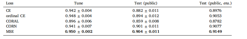
Table 5Classification performance of Local H-ViT for different loss functions, obtained with (2048, 2048) regions at 0.50 mpp. Wereport the mean and standard deviation of the quadratic weighted kappa across the 5 cross-validation folds, along with thekappa score achieved by ensembling predictions from each fold
表 5 不同损失函数下 Local H-ViT 的分类性能(采用 0.50 微米 / 像素分辨率的 2048×2048 区域)我们报告了 5 折交叉验证中加权 kappa 系数的均值和标准差,以及通过集成各折预测结果得到的 kappa 分数。
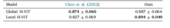
Table 6TCGA BRCA subtyping results. Both models are trained with (4096,4096) regions onthe splits from Chen et al. (2022). We report the mean and standard deviation of theAUC across the 10 cross-validation folds.
表 6 TCGA BRCA 亚型分类结果两种模型均使用(4096,4096)区域在 Chen 等人(2022)的数据集划分上进行训练。我们报告了 10 折交叉验证的 AUC(曲线下面积)均值和标准差。
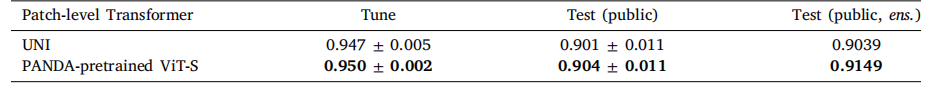
Table 7Classification performance of Local H-ViT for different feature encoders, obtained with MSE loss and (2048, 2048) regions at0.50 mpp. We report the mean and standard deviation of the quadratic weighted kappa across the 5 cross-validation folds,along with the kappa score achieved by ensembling predictions from each fold.
表 7 不同特征编码器下 Local H-ViT 的分类性能(采用 MSE 损失和 0.50 微米 / 像素分辨率的 2048×2048 区域)我们报告了 5 折交叉验证中加权 kappa 系数的均值和标准差,以及通过集成各折预测结果得到的 kappa 分数。
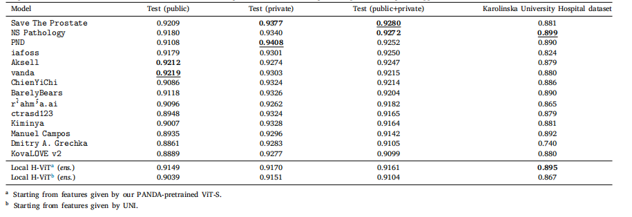
Table 8Classification performance of our best ensemble Local H-ViT models against that of PANDA consortium teams on PANDA public and private test sets, as well as Karolinska UniversityHospital dataset, used as external validation data after the challenge ended. All values are given as quadratic weighted kappa
表 8 最佳集成 Local H-ViT 模型与 PANDA 联盟团队模型的分类性能对比对比基于 PANDA 公开测试集、私有测试集以及卡罗林斯卡大学医院数据集(挑战结束后用作外部验证数据)。所有数值均以加权 kappa 系数表示。
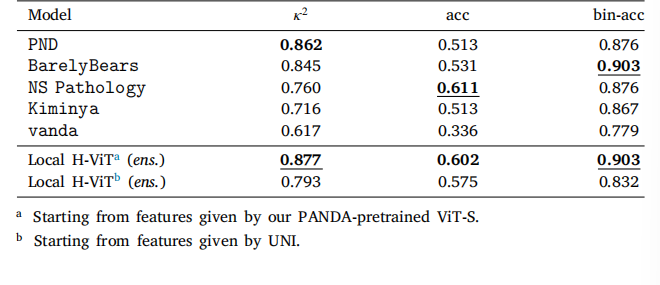
Table 9Classification performance of our ensemble Local H-ViT models compared to fivePANDA consortium teams on the crowdsourced dataset. We report quadratic weightedkappa (𝜅 2 ), overall accuracy (acc), and binary accuracy (bin-acc) for distinguishingbetween low-risk (ISUP ≤ 1) and higher-risk cases.
表 9 集成 Local H-ViT 模型与五个 PANDA 联盟团队模型在众包数据集上的分类性能对比我们报告了加权 kappa 系数(𝜅²)、总体准确率(acc)以及区分低风险(ISUP ≤ 1)与高风险病例的二元准确率(bin-acc)。
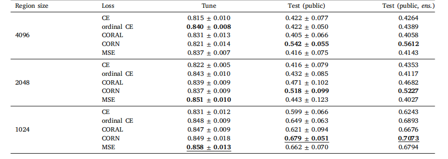
Table A.1Global H-ViT results when pretrained on TCGA dataset, for different region sizes and loss functions. We report the mean and standard deviationof the quadratic weighted kappa across the 5 cross-validation folds, along with the kappa score achieved by ensembling predictions from eachfold
表 A.1 基于 TCGA 数据集预训练的 Global H-ViT 在不同区域大小和损失函数下的结果我们报告了 5 折交叉验证中加权 kappa 系数的均值和标准差,以及通过集成各折预测结果得到的 kappa 分数
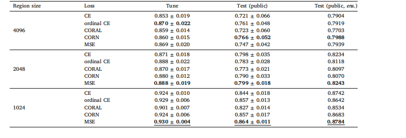
Table A.2Global H-ViT results when pretrained on PANDA dataset, for different region sizes and loss functions. We report the mean and standard deviationof the quadratic weighted kappa across the 5 cross-validation folds, along with the kappa score achieved by ensembling predictions from eachfold.
表 A.2 基于 PANDA 数据集预训练的 Global H-ViT 在不同区域大小和损失函数下的结果我们报告了 5 折交叉验证中加权 kappa 系数的均值和标准差,以及通过集成各折预测结果得到的 kappa 分数。
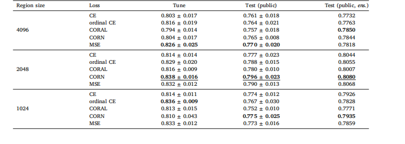
Table B.3Local H-ViT results when pretrained on TCGA dataset, for different region sizes and loss functions. We report the mean and standard deviationof the quadratic weighted kappa across the 5 cross-validation folds, along with the kappa score achieved by ensembling predictions from eachfold.
表 B.3 基于 TCGA 数据集预训练的 Local H-ViT 在不同区域大小和损失函数下的结果我们报告了 5 折交叉验证中加权 kappa 系数的均值和标准差,以及通过集成各折预测结果得到的 kappa 分数。
Table B.4Local H-ViT results when pretrained on PANDA dataset, for different region sizes and loss functions. We report the mean and standard deviationof the quadratic weighted kappa across the 5 cross-validation folds, along with the kappa score achieved by ensembling predictions from eachfold.
表 B.4 基于 PANDA 数据集预训练的 Local H-ViT 在不同区域大小和损失函数下的结果我们报告了 5 折交叉验证中加权 kappa 系数的均值和标准差,以及通过集成各折预测结果得到的 kappa 分数。
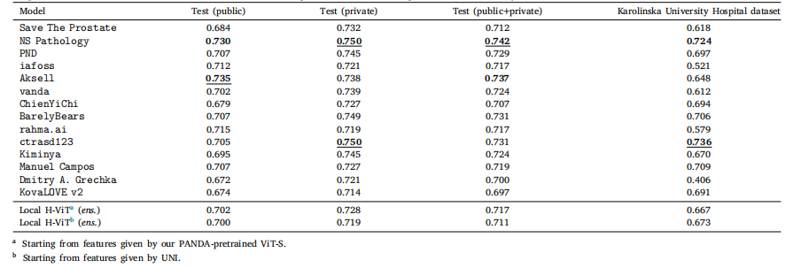
Table D.5Classification performance of our best ensemble Local H-ViT models against that of PANDA consortium teams on PANDA public and private test sets, as well as Karolinska UniversityHospital dataset, used as external validation data after the challenge ended. All values are given as overall accuracy
表 D.5 最佳集成 Local H-ViT 模型与 PANDA 联盟团队模型的分类性能对比对比基于 PANDA 公开测试集、私有测试集以及卡罗林斯卡大学医院数据集(挑战结束后用作外部验证数据)。所有数值均以整体准确率表示。
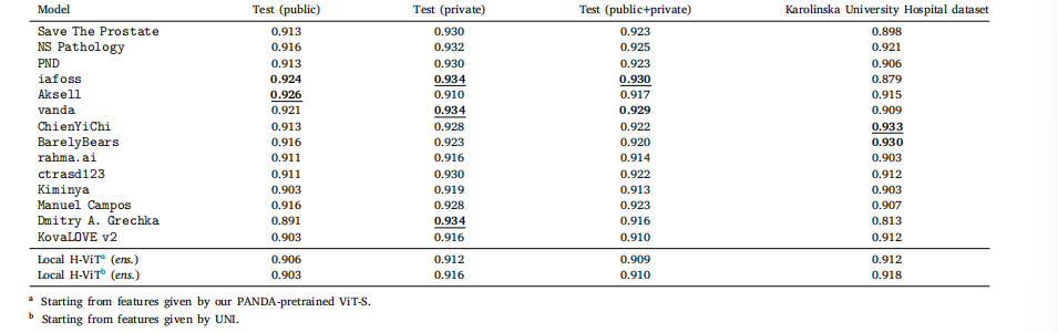
Table D.6Classification performance of our best ensemble Local H-ViT models against that of PANDA consortium teams on PANDA public and private test sets, as well as Karolinska UniversityHospital dataset, used as external validation data after the challenge ended. All values are given as binary accuracy for distinguishing between low-risk (ISUP ≤ 1) and higher-riskcases.
表 D.6 最佳集成 Local H-ViT 模型与 PANDA 联盟团队模型的分类性能对比对比基于 PANDA 公开测试集、私有测试集以及卡罗林斯卡大学医院数据集(挑战结束后用作外部验证数据)。所有数值均以区分低风险(ISUP ≤ 1)与高风险病例的二元准确率表示。
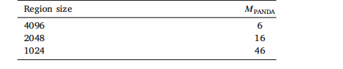
Table E.7Average number of regions per slide, PANDA dataset
表 E.7 PANDA 数据集中每张切片的平均区域数量
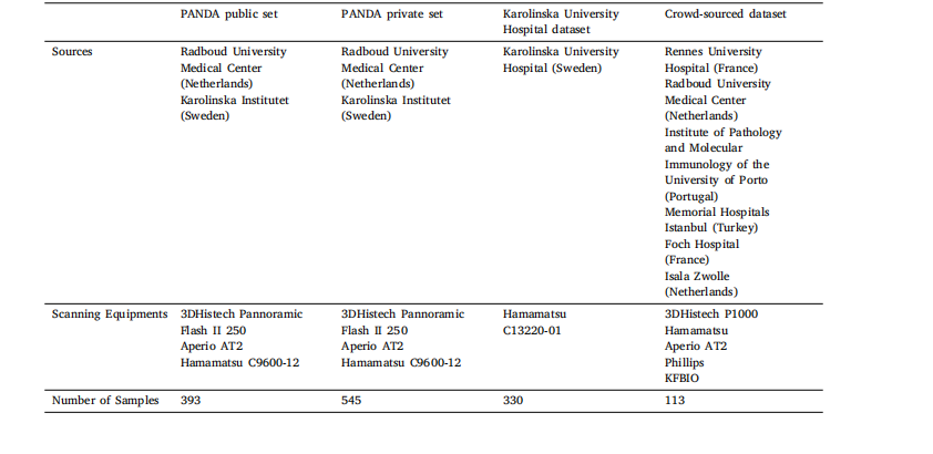
Table F.8Test datasets details.
表 F.8 测试数据集详情
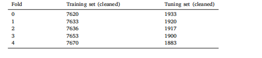
Table G.9Number of slide per partition after label denoising, 5-fold CV splits.
表 G.9 标签去噪后各划分中的切片数量(5 折交叉验证分割)

Table J.10Global H-ViT results when pretrained on PANDA dataset with (2048, 2048) regions, for different loss functions. We report quadratic weightedkappa averaged over the 5 cross-validation folds (mean ± std)
表 J.10 基于 PANDA 数据集预训练的 Global H-ViT 在不同损失函数下的结果(采用 2048×2048 区域)我们报告了 5 折交叉验证中加权 kappa 系数的平均值(± 标准差)。
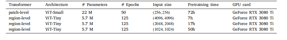
Table L.11Computational characteristics of DINO pretraining of the path-level and region-level Transformer on PANDA.
表 L.11 PANDA 数据集上路径级和区域级 Transformer 的 DINO 预训练计算特征

Table L.12Comparison of number of trainable parameters, training time, and GPU memory usage for Global H-ViT and Local H-ViT.
表 L.12 Global H-ViT 与 Local H-ViT 的可训练参数数量、训练时间及 GPU 内存使用量对比
)


)


)
的编程实现方法:1、数据包格式定义结构体2、使用队列进行数据接收、校验解包)

)


——标准库函数大全(持续更新))