BisenetV1/2网络以及模型推理转换

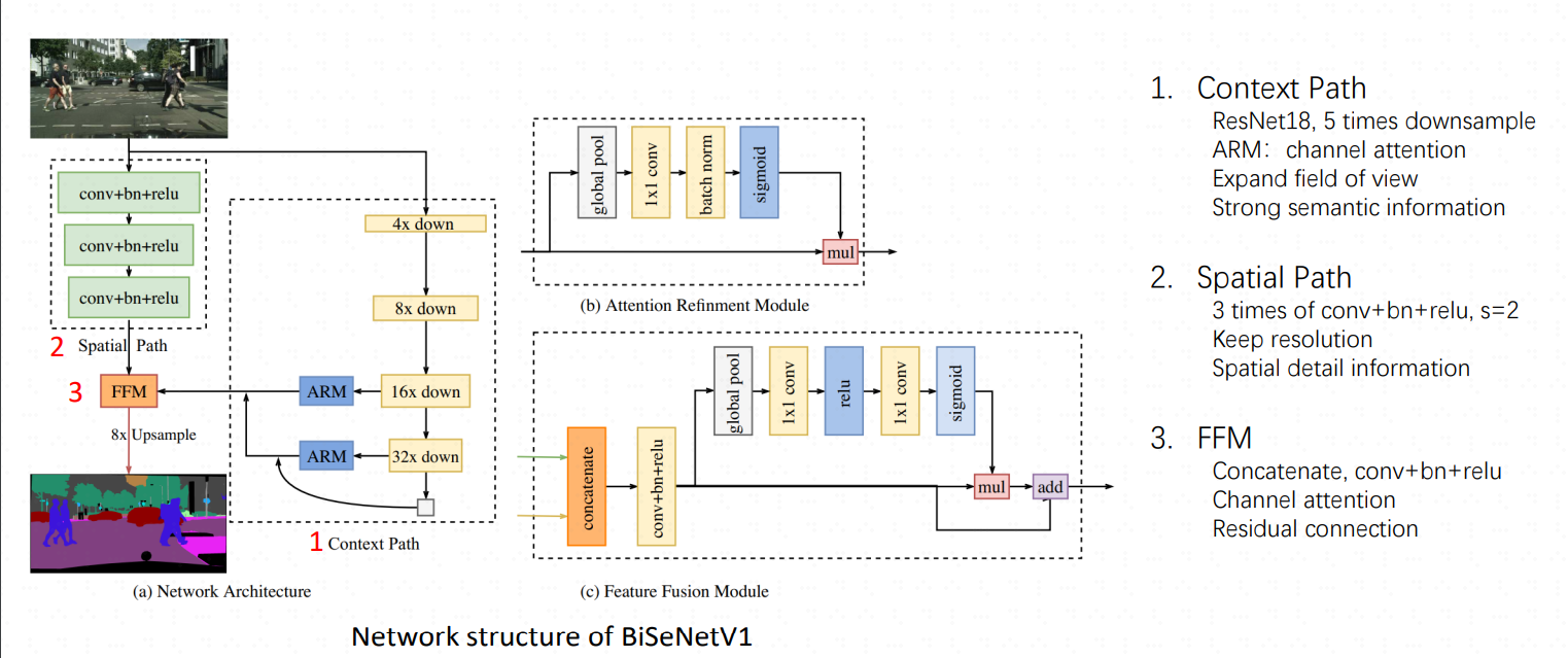
1 BiSenetV1

相关开源地址，eg1，

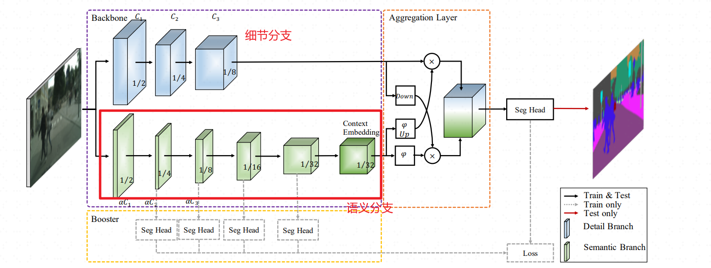
  为了加速模型推理，很多模型裁剪图像尺寸、剪枝卷积网络通道、卷积步骤数等，这样损失了空间信息以及相应的感受野，BiSenet这个网络选择融合SP和CP两个通道来实现加速

class BiSeNetV1(nn.Module):def __init__(self, n_classes, aux_mode='train', *args, **kwargs):super(BiSeNetV1, self).__init__()self.cp = ContextPath()self.sp = SpatialPath()self.ffm = FeatureFusionModule(256, 256)self.conv_out = BiSeNetOutput(256, 256, n_classes, up_factor=8)self.aux_mode = aux_modeif self.aux_mode == 'train':self.conv_out16 = BiSeNetOutput(128, 64, n_classes, up_factor=8)self.conv_out32 = BiSeNetOutput(128, 64, n_classes, up_factor=16)self.init_weight()def forward(self, x):H, W = x.size()[2:]feat_cp8, feat_cp16 = self.cp(x)feat_sp = self.sp(x)feat_fuse = self.ffm(feat_sp, feat_cp8)feat_out = self.conv_out(feat_fuse)if self.aux_mode == 'train':feat_out16 = self.conv_out16(feat_cp8)feat_out32 = self.conv_out32(feat_cp16)return feat_out, feat_out16, feat_out32elif self.aux_mode == 'eval':return feat_out,elif self.aux_mode == 'pred':#  feat_out = feat_out.argmax(dim=1)feat_out = CustomArgMax.apply(feat_out, 1)return feat_outelse:raise NotImplementedErrordef init_weight(self):for ly in self.children():if isinstance(ly, nn.Conv2d):nn.init.kaiming_normal_(ly.weight, a=1)if not ly.bias is None: nn.init.constant_(ly.bias, 0)def get_params(self):wd_params, nowd_params, lr_mul_wd_params, lr_mul_nowd_params = [], [], [], []for name, child in self.named_children():child_wd_params, child_nowd_params = child.get_params()if isinstance(child, (FeatureFusionModule, BiSeNetOutput)):lr_mul_wd_params += child_wd_paramslr_mul_nowd_params += child_nowd_paramselse:wd_params += child_wd_paramsnowd_params += child_nowd_paramsreturn wd_params, nowd_params, lr_mul_wd_params, lr_mul_nowd_params

1.1 Contex Path

  上下文通道是的backbone基于Resnet18去实现的

# 上下文path
class ContextPath(nn.Module):def __init__(self, *args, **kwargs):super(ContextPath, self).__init__()self.resnet = Resnet18()        # 调用残差网络  resnet.pyself.arm16 = AttentionRefinementModule(256, 128)self.arm32 = AttentionRefinementModule(512, 128)self.conv_head32 = ConvBNReLU(128, 128, ks=3, stride=1, padding=1)self.conv_head16 = ConvBNReLU(128, 128, ks=3, stride=1, padding=1)self.conv_avg = ConvBNReLU(512, 128, ks=1, stride=1, padding=0)self.up32 = nn.Upsample(scale_factor=2.)self.up16 = nn.Upsample(scale_factor=2.)self.init_weight()def forward(self, x):# 下采样的特征是通过残差网络Resnet18得到的feat8, feat16, feat32 = self.resnet(x)avg = torch.mean(feat32, dim=(2, 3), keepdim=True)avg = self.conv_avg(avg)feat32_arm = self.arm32(feat32)feat32_sum = feat32_arm + avgfeat32_up = self.up32(feat32_sum)   # 原来下采样，现在上采样恢复feat32_up = self.conv_head32(feat32_up)feat16_arm = self.arm16(feat16)feat16_sum = feat16_arm + feat32_up         # 两次采样相加feat16_up = self.up16(feat16_sum)feat16_up = self.conv_head16(feat16_up)return feat16_up, feat32_up # x8, x16    feat16_up就是最终的输出

1.2 Spatial Path

空间通道比较简单

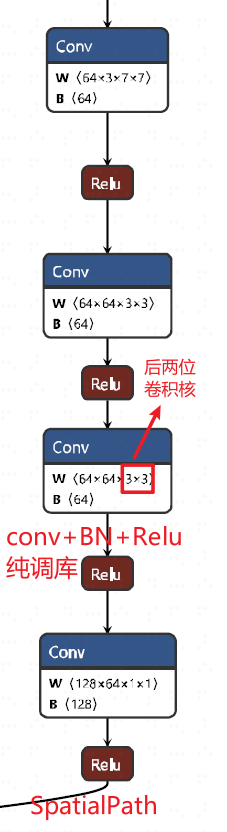
class SpatialPath(nn.Module):def __init__(self, *args, **kwargs):# super() 函数用于调用父类nn.Module的方法，这里调用了调用了 nn.Module 的构造函数# super() 函数的第一个参数是当前类（SpatialPath）# super() 第二个参数是当前类的实例（self）super(SpatialPath, self).__init__()     self.conv1 = ConvBNReLU(3, 64, ks=7, stride=2, padding=3)           # 卷积核大小为7x7，步长为2，填充为3self.conv2 = ConvBNReLU(64, 64, ks=3, stride=2, padding=1)self.conv3 = ConvBNReLU(64, 64, ks=3, stride=2, padding=1)self.conv_out = ConvBNReLU(64, 128, ks=1, stride=1, padding=0)self.init_weight()      # 初始化权重def forward(self, x):       # x 是输入数据，通常是一个四维张量，形状为 (batch_size, channels, height, width)# 定义前向传播过程----卷积计算feat = self.conv1(x)feat = self.conv2(feat)feat = self.conv3(feat)feat = self.conv_out(feat)return feat

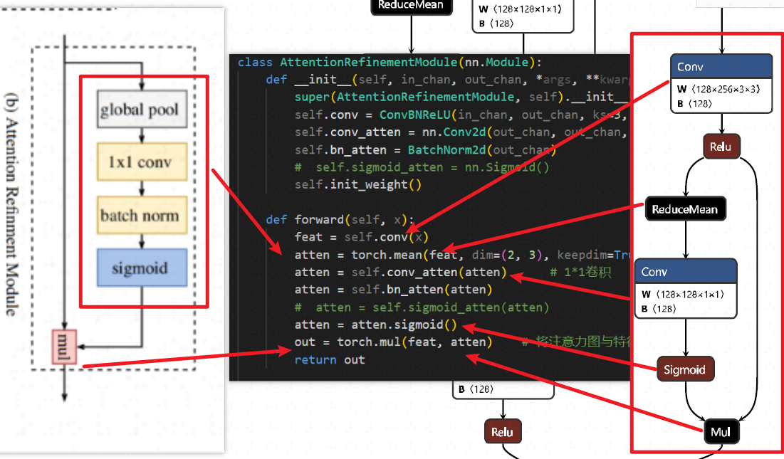
1.3 ARM

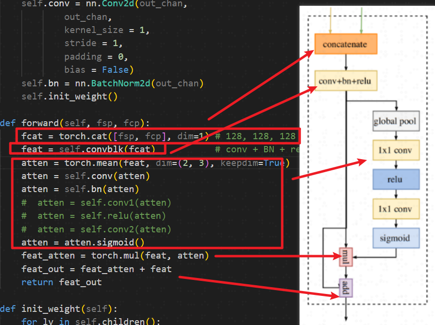
1.4 FFM

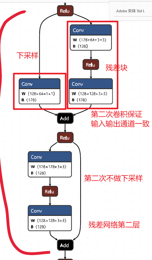
1.5 backbone

这里使用的是resnet网络，可视化残差网络第二层

2 模型推理代码流程分析

2.1 加载模型

net = model_factory[cfg.model_type](cfg.n_cats, aux_mode='eval')
net.load_state_dict(torch.load(args.weight_path, map_location='cpu'), strict=False)
net.eval()     # 设置为推理模式
net.cuda()     # 将模型加载到GPU上

2.2 模型推理

① 转换张量

对于一张图像

# prepare data
to_tensor = T.ToTensor(mean=(0.3257, 0.3690, 0.3223), # city, rgbstd=(0.2112, 0.2148, 0.2115),
)
im = cv2.imread(args.img_path)[:, :, ::-1]   # [:, :, ::-1] 将 BGR 格式转换为 RGB（因 OpenCV 默认读取为 BGR，而PyTorch需要 RGB）
im = to_tensor(dict(im=im, lb=None))['im'].unsqueeze(0).cuda()      # 按均值 mean=(0.3257, 0.3690, 0.3223) 和标准差 std=(0.2112, 0.2148, 0.2115) 对图像进行标准化（逐通道操作）# PyTorch 模型通常接受批处理输入（即使只有一张图像），格式为 [B, C, H, W]。如果没有 unsqueeze(0)，模型会因维度不匹配而报错。假设输入图像经过 ToTensor 转换后的形状是 [C, H, W]（通道、高度、宽度）：原始 Tensor：(3, 224, 224) （RGB 图像，3 通道，224x224 分辨率）
unsqueeze(0) 后：(1, 3, 224, 224) （添加了 batch 维度，表示 batch_size=1）

对于视频流，那么这里的B就会变大，比如一次处理列表里面的8帧，就是一个批次8帧

② 输入尺寸调整

im = F.interpolate(im, size=new_size, align_corners=False, mode='bilinear')

• 作用：将输入图像 im 的尺寸调整为 new_size（之前计算的32的倍数，如 512x704）。
• 参数说明：
  • size=new_size：目标尺寸（高度和宽度）。
  • mode='bilinear'：使用双线性插值（平衡速度和质量）。
  • align_corners=False：避免边缘像素对齐问题（推荐设置）。
• 为什么需要调整输入尺寸？
  确保输入尺寸符合模型的架构要求（如全卷积网络需要尺寸能被下采样因子整除）。

---

③ 模型推理

out = net(im)[0]

• 作用：将调整后的图像输入模型 net，获取输出。

• [0] 的含义：

  如果模型返回多个输出（如主输出 + 辅助头输出），[0]表示只取主输出。例如：

  • 输出形状可能是 [B, C, H, W]（Batch, 类别数, 高, 宽）。
  • 若 B=1（单张图像），out 的形状为 [C, H, W]。

---

④ 输出尺寸还原

out = F.interpolate(out, size=org_size, align_corners=False, mode='bilinear')

• 作用：将模型输出的特征图 out 插值回原始图像尺寸 org_size（如 480x640）。
• 为什么需要还原尺寸？
  • 模型输出的分辨率通常比输入低（因下采样），需还原到原始尺寸以便后续处理（如可视化或评估）。
  • 例如：
    • 输入尺寸：512x704 → 模型输出：16x22（下采样32倍）→ 插值回 480x640。

---

⑤ 类别预测

out = out.argmax(dim=1)		# 张量模式，每一个像素值都是一种类别，用相应的数字表示！

• 作用：对特征图 out 沿 类别维度（dim=1） 取 argmax，得到每个像素的预测类别。
• 输入输出形状：
  • 输入 out：[C, H, W]（C是类别数，如分割任务有20类）。
  • 输出 out：[H, W]，每个像素值为 0 到 C-1 的整数（表示类别ID）。
• 示例：
  如果 C=3（3类：背景、猫、狗），out 的每个像素值会是 0、1 或 2。

---

⑥ 保存绘制

先转换张量

out = out.squeeze().detach().cpu().numpy()      # 将张量转换为NumPy数组
pred = palette[out]# 生成256*3的数组，每个数处于0-255之间
palette = np.random.randint(0, 256, (256, 3), dtype=np.uint8)		# 一个预定义的调色板（颜色映射表），形状为 [num_classes, 3]，等价下面
palette = np.array([		[0, 0, 0],      # 类别0：黑色（背景）[255, 0, 0],    # 类别1：红色（猫）[0, 255, 0],    # 类别2：绿色（狗）# ...其他类别颜色
], dtype=np.uint8)

⑦ 关于视频流

[视频文件]|v
生产者进程 ──(in_q)──> 主进程 ──(out_q)──> 消费者进程|                      |                    || (帧: [1,3,1080,1920])| (结果: [1,1080,1920])|v                      v                    v预处理                [GPU批量推理]           保存为MP4|                      |v                      v
BGR→RGB              合并8帧→[8,3,768,768]|                      |v                      v
Tensor化             缩放→推理→还原分辨率

3 pth转onnx

3.1 为什么要转换

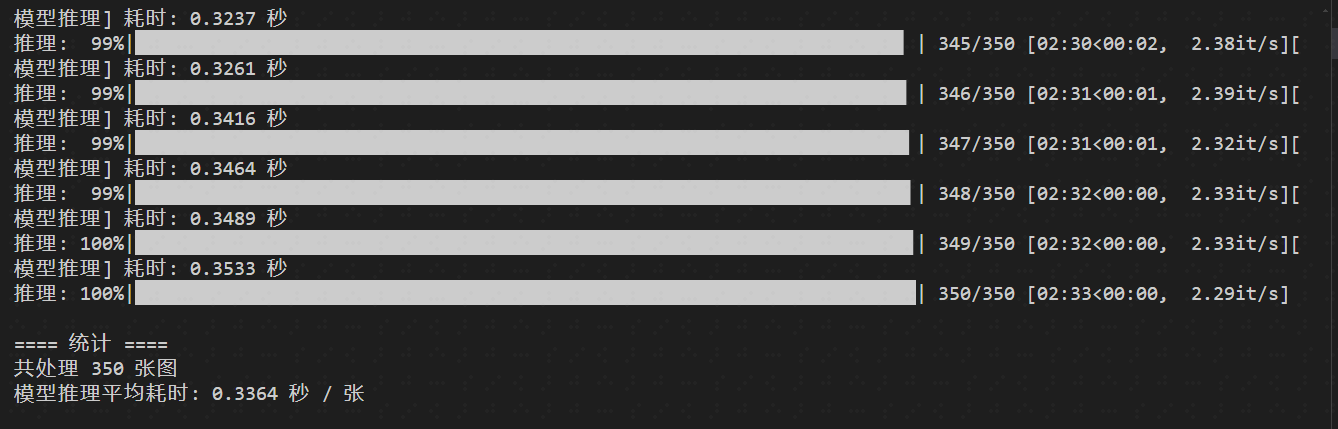
pth这种权重加载时候需要定义具体的网络模型，而onnx则不需要。而且pth每一次推理耗时会更久，但onnx则每一次减少一半以上

所以这里把pth权重转换为onnx

(segment) D:\wpj\Bisnetv1>python tools/demo.py --config configs/bisenetv1_ipm0121.py --weight-path res/IPM0121/model_epoch_21.pth --img-path ./datasets/ipm_all_annoted_0121/images/training/0112.jpg
[张量] 耗时: 0.0000 秒
[图像读取与预处理] 耗时: 0.0036 秒
[图像转化为tensor] 耗时: 0.0180 秒
[推理：] 耗时: 0.7578 秒					# 耗时在0.75-0.8s
[预测：] 耗时: 0.0001 秒

3.2 转换代码

① 整个onnx模型导出还是需要借助BiSenetV1网络模型，配置文件也是需要的

② 设置基本的输入输出，以及算子版本

torch.set_grad_enabled(False)parse = argparse.ArgumentParser()
parse.add_argument('--config', dest='config', type=str,default='configs/bisenetv2.py',)
parse.add_argument('--weight-path', dest='weight_pth', type=str,default='model_final.pth')
parse.add_argument('--outpath', dest='out_pth', type=str,default='model.onnx')
parse.add_argument('--aux-mode', dest='aux_mode', type=str,						# 注意，preddefault='pred')
args = parse.parse_args()
cfg = set_cfg_from_file(args.config)											# 加载配置文件
if cfg.use_sync_bn: cfg.use_sync_bn = False						net = model_factory[cfg.model_type](cfg.n_cats, aux_mode=args.aux_mode)			# 定义Bisenet网络模型，用了aux_mode，会指定pred对应的argmax函数，所以说这里有可能报错，如果你的模型不指定这个，估计就不会调用这个；所以今天遇到的问题，最简单解决方式，应该是把aux_mode设置为eval模式，直接返回输出！！！！
net.load_state_dict(torch.load(args.weight_pth, map_location='cpu',				weights_only=True), strict=False)				# 加载权重	
net.eval()dummy_input = torch.randn(1, 3, *cfg.cropsize)							#  dummy_input = torch.randn(1, 3, 1024, 1024)
input_names = ['input_image']											# 输入和输出，以及dynamic_axes设置形式一般这样
output_names = ['preds']
dynamic_axes = {'input_image': {0: 'batch'}, 'preds': {0: 'batch'}}		# 指定模型的哪些输入/输出维度是动态的torch.onnx.export(net, dummy_input, 						# 输入args.out_pth,						# 输出路径input_names=input_names, 			# 输入名output_names=output_names,			# 输出名verbose=False, opset_version=16,                   #  算子集版本原来是18，不兼容这个pytorch版本，改成16---这里pytorch-1.13# operator_export_type=torch.onnx.OperatorExportTypes.ONNX,dynamic_axes=dynamic_axes)

③ 一直报错是关于BiSeNetV1网络中forward函数中关于CustomArgMax的调用，这个CustomArgMax是一个自定义的argmax（在对一系列类别预测中，选择概率最大的哪一个），在train和pred模式下是没有调用，故此没有问题；但是在转换模型，即为pred模式下，发生了错误！因为它在symbolic返回中填的错误算子，系统找不到！

④ 定义Bisenet网络模型，用了aux_mode，会指定pred对应的argmax函数，所以说这里有可能报错，如果你的模型不指定这个，估计就不会调用这个；所以今天遇到的问题，最简单解决方式，应该是把aux_mode设置为eval模式，直接返回输出！经过实验，确实如此！！因为他写的CustomArgMax存在问题，eval是后面修改过的函数！！

class BiSeNetV1(nn.Module):def __init__(self, n_classes, aux_mode='train', *args, **kwargs):super(BiSeNetV1, self).__init__()......def forward(self, x):H, W = x.size()[2:]feat_cp8, feat_cp16 = self.cp(x)feat_sp = self.sp(x)feat_fuse = self.ffm(feat_sp, feat_cp8)feat_out = self.conv_out(feat_fuse)if self.aux_mode == 'train':feat_out16 = self.conv_out16(feat_cp8)feat_out32 = self.conv_out32(feat_cp16)return feat_out, feat_out16, feat_out32elif self.aux_mode == 'eval':return feat_out,elif self.aux_mode == 'pred':#  feat_out = feat_out.argmax(dim=1)feat_out = CustomArgMax.apply(feat_out, 1)return feat_outelse:raise NotImplementedErrorclass CustomArgMax(torch.autograd.Function):@staticmethoddef forward(ctx, feat_out, dim):if torch.onnx.is_in_onnx_export():# ONNX导出时：返回原始logits（保持梯度流）ctx.mark_dirty(feat_out)  # 避免警告return feat_out# 训练/推理时：正常执行argmaxreturn feat_out.argmax(dim=dim).int()				# 实际上，pred应该也可以使用argmax，在推理时候就不可以使用了！！@staticmethoddef symbolic(g, feat_out, dim: int):# 导出为Identity节点（避免引入ArgMax）return g.op("Identity", feat_out)			# 原始代码return g.op('CustomArgMax', feat_out, dim_i=dim)，这里执行不了         

3.3 转换测试

python ./tools/xx.py --config configs/xx.py --weight-path ./res/x/x.pth

可视化模型，忘记放代码了，后面补一下

python ./tools/x.py		# 可视化onnx权重，打印输入输出形状# Dtype: 1   Dtype 是 Data Type 的缩写，代表张量的数据类型。  eg, 1	torch.float32    2	torch.float64
===== Inputs =====
Name: input_image, Shape: ['batch', 3, 1024, 1024], Dtype: 1===== Outputs =====
Name: preds, Shape: ['batch', 2, 1024, 1024], Dtype: 1		# 2是类别数

推理测试 ，推理测试代码待补充

python ./tools/x.py --config configs/xxx.py --weight-path ./model.onnx --img-path ./datasets/xxx/x.jpg		# 推理一张

python ./tools/xx.py		# 推理一个文件内的所有IPM图像

4 onnx转MNN

4.1 编译MNN库

下载MNN库，为了转换

git clone https://github.com/alibaba/MNN.git
cd MNN
mkdir build && cd build
cmake .. -DMNN_BUILD_CONVERTER=ON -DMNN_OPENCL=ON -DMNN_VULKAN=ON  # opencl是为了GPU推理
make -j$(nproc)			# 工具位于 ./build/MNNConvert
sudo make install

./MNNConvert -f ONNX --modelFile xxx.onnx --MNNModel xxx.mnn ./MNNConvert --framework=ONNX --model=your_model.onnx --MNNModel=output.mnn --optimizeLevel=3 感觉没啥用 --bizCode=your_code 版权-f ONNX	指定输入模型格式为 ONNX
--modelFile	输入模型的路径（这里是 model.onnx）	
--MNNModel	输出模型的路径（转换后的 MNN 模型保存为 model.mnn）	--fp16	启用 FP16 量化（减小模型体积，提升推理速度，可能损失少量精度）
--weightQuantBits 8	INT8 权重量化（进一步压缩模型，需校准数据）
--optimizeLevel 2	优化级别（0不优化，1基础优化，2激进优化，可能改变计算图结构）
--inputConfigFile	指定动态输入的形状（通过 JSON 文件配置，解决 None 维度问题）
--forTraining	保留训练相关算子（默认转为推理模型）
--saveStaticModel	固定输入形状（移除动态维度，提升推理性能）

4.2 模型推理测试

  关于c++调用MNN模型的代码还是有很多坑的（python代码比较简单），官方文档中例子也给的很奇怪，代码后续给出来

5 BisenetV2测试

   BisenetV2优势在于用更加轻量模块来替换V1中原有Backbone即Resnet-18网络。论文中V2的速度应该是156 FPS / 65 FPS ≈ 2.4于V1。但实际测试完全达不到论文结果，原始论文代码未开源，论文中关于网络细节不像V1清楚，搜索发现网上复现达不到论文效果。

板卡测试—8核 –ubunt20.04------mnn模型

V2（13 MB）相较于 V1（50 MB）参数量下降，但计算貌似没有太大区别----因此不同模型的参数量不能直接作为推理速度标准，只可参考

单线程下V2（682 ms）快于V1网络（840 ms）158 ms

2线程下V2（435 ms）快于V1网络（481 ms）46 ms

4线程下V2（356 ms）快于V1网络（370 ms）14 ms

8线程下V2（363 ms）慢于V1网络（351 ms）11 ms

6 tee工具

  在测试过程中发现，想要保存终端打印的信息，又不想自己写保存代码，还得编译cpp，找到tee这个工具，可以在linux终端命令行执行时，捕捉终端打印记录并保存，还是很好用的。

python test.py  2>&1 | tee output.txt