视觉SLAM第7讲：视觉里程计2（3D-2D:PnP、3D-3D:ICP）

接上文，视觉SLAM第7讲：视觉里程计1（特征点法、2D-2D对极约束），本节主要学习3D-2D:PnP、3D-3D:ICP。

目录

7.7 3D-2D:PnP

7.7.1 直接线性变换（DLT）

7.7.2 P3P

1.原理

2.小结

7.7.3 最小化重投影误差求解PnP

1.引言

2.原理

7.8 实践：求解PnP

7.8.1 使用EPnP求解位姿（调用OpenCV库）

7.8.2 手写位姿估计

7.8.3 使用g2o进行BA优化

7.8.4 报错修复

1.报错代码

2.检查与修复

7.9 3D-3D：ICP

7.9.1 SVD法（线性代数求解）

7.9.2 非线性优化方法

7.10 实践：求解ICP

7.10.1 实践：SVD方法

1.pose_estimation_3d3d.cpp

2.CmakeLists.txt

3.运行结果

7.10.2 实践非线性优化方法

1.涉及代码

2.运行结果

7.11 小结

7.7 3D-2D:PnP

PnP(Perspective-n-Point)是求解3D到2D点对运动的方法。它描述了当知道n个3D空间点及其投影位置时，如何估计相机的位姿（外参，平移和旋转）。2D-2D 的对极几何方法需要8个或8个以上的点对(以八点法为例)，且存在着初始化、纯旋转和尺度的问题。然而，如果两张图像中的一张特征点的3D位置已知，那么最少只需3个点对(以及至少一个额外点验证结果)就可以估计相机运动。

特征点的3D位置可以由三角化或者RGB-D相机的深度图确定。因此，在双目或RGB-D的视觉里程计中，我们可以直接使用PnP估计相机运动，3D-2D方法不需要使用对极约束，又可以在很少的匹配点中获得较好的运动估计，是一种最重要的姿态估计方法；而在单目视觉里程计中，必须先进行初始化，才能使用PnP。
PnP问题有很多种求解方法，例如，用3对点估计位姿的P3P、直接线性变换(DLT)，EPnP(Efficient PnP)、UPnP等等。此外，还能用非线性优化的方式，构建最小二乘问题并迭代求解，也就是万金油式的光束法平差(Bundle Adjustment，BA)。

7.7.1 直接线性变换（DLT）

已知一组3D点的位置，以及它们在某个相机中的投影位置，求该相机的位姿。这个问题也可以用于求解给定地图和图像时的相机状态问题。如果把3D点看成在另一个相机坐标系中的点的话，则也可以用来求解两个相机的相对运动问题。
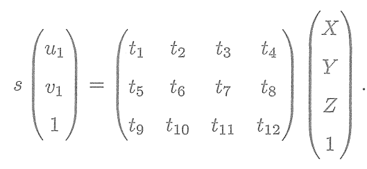
考虑某个空间点 $P$ ，它的齐次坐标为 $P=(X,Y,Z,1)^{T}$ 。在图像中 $I_{1}$ ，投影到特征点 $x_{1}=(u_{1},v_{1},1)^{T}$ (以归一化平面齐次坐标表示)。此时，相机的位姿 $R,t$ 是未知的。与单应矩阵的求解类似，我们定义增广矩阵 $[R|t]$ 为一个3×4的矩阵，包含了旋转与平移信息，展开形式为



消去 $s$ ，得到两个约束：

   $u_{1}=\frac{t_{1}X+t_{2}Y+t_{3}Z+t_{4}}{t_{9}X+t_{10}Y+t_{11}Z+t_{12}},v_{1}=\frac{t_{5}X+t_{6}Y+t_{7}Z+t_{8}}{t_{9}X+t_{10}Y+t_{11}Z+t_{12}}$

为了简化表示，定义 $T$ 的行向量：

   $t_{1}=(t_{1},t_{2},t_{3},t_{4})^{T},t_{2}=(t_{5},t_{6},t_{7},t_{8})^{T},t_{3}=(t_{9},t_{10},t_{11},t_{12})^{T}$

于是有：

   $t_{1}^{T}P-t_{3}^{T}Pu_{1}=0,t_{2}^{T}P-t_{3}^{T}Pv_{1}=0$
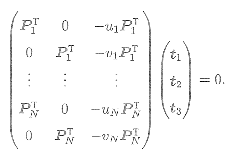
$t$ 是待求的变量，每个特征点提供了两个关于 $t$ 的线性约束。假设一共有 $N$ 个特征点，则可以列出如下线性方程组：



   $t$ 一共有12维，因此最少通过6对匹配点即可实现矩阵T的线性求解，这种方法称为DLT。当匹配点大于6对时，也可以使用SVD等方法对超定方程求最小二乘解。

在DLT求解中，我们直接将T矩阵看成了12个未知数，忽略了它们之间的联系。因为旋转矩阵R∈ SO(3)，用DLT求出的解不一定满足该约束，它是一个一般矩阵。

平移向量比较好办，它属于向量空间。

对于旋转矩阵R，我们必须针对DLT估计的T左边3×3的矩阵块，寻找一个最好的旋转矩阵对它进行近似。这可以由QR分解完成，也可以像这样来计算： $R\leftarrow (R^R{T})^{-\frac{1}{2}}R$
这相当于把结果从矩阵空间重新投影到SE(3)流形上，转换成旋转和平移两部分。
这里的 $x_{1}$ 使用归一化平面坐标，去掉了内参矩阵K的影响——这是因为内参在SLAM中通常假设为已知。即使内参未知，也能用PnP去估计 $K,R,t$ 三个量。然而由于未知量增多，效果会差一些。

7.7.2 P3P

1.原理

P3P是另一种解PnP的方法，它仅使用3对匹配点，对数据要求较少。
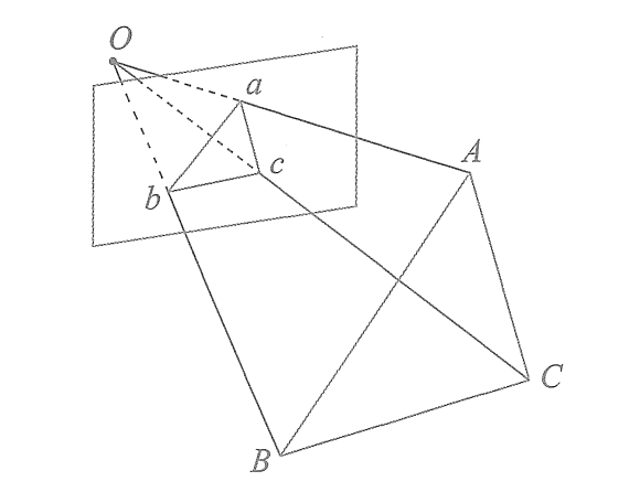
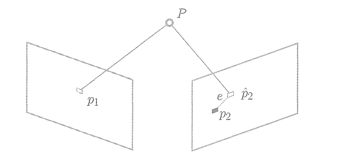
P3P需要利用给定的3个点的几何关系。它的输入数据为3对3D-2D匹配点。记3D点为A、B、C（世界坐标系中），2D点为a、b、c，其中小写字母代表的点为对应大写字母代表的点在相机成像平面上的投影，如下图。此外，P3P还需要使用一对验证点，以从可能的解中选出正确的那一个(类似于对极几何情形)。记验证点对为D-d，相机光心为O。

一旦3D点在相机坐标系下的坐标能够算出，我们就得到了3D-3D的对应点，把PnP问题转换为了ICP问题。

三角形之间存在对应关系： $\Delta Oab-\Delta OAB,\Delta Obc-\Delta OBC,\Delta Oac-\Delta OAC$

考虑Oab和OAB的关系。利用余弦定理，有

$OA^{2}+OB^{2}-2OA·OBcos<a,b>=AB^{2}$

对于其他两个三角形也有类似性质，于是有：

$OB^{2}+OC^{2}-2OB·OCcos<b,c>=BC^{2}$

$OA^{2}+OC^{2}-2OA·OCcos<a,c>=AC^{2}$

对以上三式全体除以 $OC^{2}$ ，并且记 $x=OA/OC,y=OB/OC$ ，

得：

   $x^{2}+y^{2}-2xycos<a,b>=\frac{AC^{2}}{OC^{2}}$

   $y^{2}+1^{2}-2ycos<b,c>=\frac{BC^{2}}{OC^{2}}$

   $x^{2}+1^{2}-2xcos<a,c>=\frac{AC^{2}}{OC^{2}}$

记 $v=\frac{AB^{2}}{OC^{2}},uv=\frac{BC^{2}}{OC^{2}},wv=\frac{AC^{2}}{OC^{2}}$ ，

有：

   $x^{2}+y^{2}-2xycos<a,b>-v=0$

$y^{2}+1^{2}-2ycos<b,c>-uv=0$

   $x^{2}+1^{2}-2xcos<a,c>-wv=0$

化简得：

$(1-u)y^{2}-ux^{2}-cos<b,c>y+2uxycos<a,b>+1=0$

   $(1-w)x^{2}-wy^{2}-cos<a,c>x+2wxycos<a,b>+1=0$

2D点的图像位置，3个余弦角已知； $u,w$ 可以通过 $A,B,C$ 在世界坐标系下的坐标算出，变换到相机坐标系下之后，这个比值并不改变。 $x,y$ 未知，随着相机移动会发生变化。

因此，该方程组是关于的一个二元二次方程（多项式方程)。求该方程组的解析解是一个复杂的过程，需要用吴消元法。类似于分解E的情况，该方程最多可能得到4个解，可以用验证点来计算最可能的解，得到 $A,B,C$ 在相机坐标系下的3D坐标。然后，根据3D-3D的点对，计算相机的运动 $R,t$ 。

2.小结

从P3P的原理可以看出，为了求解 PnP，利用三角形相似性，求解投影点 $a,b,c$ 在相机坐标系下的3D坐标，最后把问题转换成一个3D到3D的位姿估计问题。在后文中将看到,
带有匹配信息的3D-3D位姿求解非常容易，所以这种思路是非常有效的。一些其他的方法，例如EPnP，也采用了这种思路。

然而，P3P也存在着一些问题：

（1）P3P只利用3个点的信息。当给定的配对点多于3组时，难以利用更多的信息。

（2）如果3D点或2D点受噪声影响，或者存在误匹配，则算法失效。
所以，人们还陆续提出了许多别的方法，如EPnP、UPnP等。它们利用更多的信息，而且用迭代的方式对相机位姿进行优化，以尽可能地消除噪声的影响。在SLAM中，通常的做法是先使用P3P/EPnP等方法估计相机位姿，再构建最小二乘优化问题对估计值进行调整(即进行Bundle Adjustment )。在相机运动足够连续时，也可以假设相机不动或匀速运动，用推测值作为初始值进行优化。接下来，我们从非线性优化的角度来看PnP问题。

7.7.3 最小化重投影误差求解PnP

1.引言

除了使用线性方法，我们还可以把PnP问题构建成一个关于重投影误差的非线性最小二乘问题。

线性方法，是先求相机位姿，再求空间点位置；非线性优化则是把它们都看成优化变量，放在一起优化，这是一种非常通用的求解方式，可以用它对PnP或ICP给出的结果进行优化，这一类把相机和三维点放在一起进行最小化的问题，统称为Bundle Adjustment。
在PnP中构建一个Bundle Adjustment问题对相机位姿进行优化。如果相机是连续运动的(比如大多数SLAM过程)，也可以直接用BA求解相机位姿。我们将在本节给出此问题在两个视图下的基本形式，然后在第9讲讨论较大规模的BA问题。

2.原理

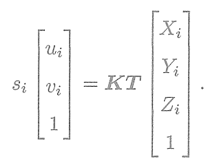
考虑 $n$ 个三维空间点 $P$ 及其投影 $p$ ，计算相机的位姿 $R,t$ ，它的李群表示为 $T$ 。假设某空间点坐标为 $P_{i}=[X_{i},Y_{i},Z_{i}]^{T}$ ，其投影的像素坐标为 $u_{i}=[u_{i},v_{i}]^{T}$ 。根据第5讲的内容，像素位置与空间点位置的关系为：

矩阵形式为： $s_{i}u_{i}=KTP_{i}$

这个式子隐含了一次从齐次坐标到非齐次的转换，否则按矩阵的乘法来说，维度是不对的。现在，由于相机位姿未知及观测点的噪声，该等式存在一个误差。因此，我们把误差求和，构建最小二乘问题，然后寻找最好的相机位姿，使它最小化：

   $T^{*}=argmin_{T}\frac{1}{2}\sum_{i=1}^{n}||u_{i}-\frac{1}{s_{i}}KTP_{i}||_{2}^{2}$
该问题的误差项，是将3D点的投影位置与观测位置作差，所以称为重投影误差。使用齐次坐标时，这个误差有3维。不过，由于 $u$ 最后一维为1，该维度的误差一直为零，因而我们更多时候使用非齐次坐标，于是误差就只有2维了。

如图所示，我们通过特征匹配知道了 $p_{1}$ 和 $p_{2}$ 是同一个空间点 $P$ 的投影，但是不知道相机的位姿。在初始值中， $P$ 的投影 $\hat{p_{2}}$ 与实际的 $p_{2}$ 之间有一定的距离。于是我们调整相机的位姿，使得这个距离变小。不过，由于这个调整需要考虑很多个点，所以最后的效果是整体误差的缩小，而每个点的误差通常都不会精确为零。

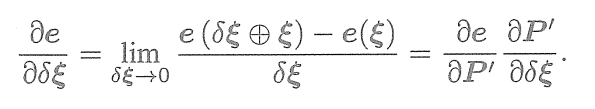
使用李代数，可以构建无约束的优化问题，很方便地通过高斯牛顿法、列文伯格-马夸尔特方法等优化算法进行求解。不过，在使用高斯牛顿法和列文伯格-马夸尔特方法之前，我们需要知道每个误差项关于优化变量的导数，也就是线性化： $e(x+\Delta x)\approx e(x)+J^{T}\Delta x$

$J^{T}$ 的形式是关键所在。我们固然可以使用数值导数，但如果能够推导出解析形式，则优先考虑解析导数。现在，当 $e$ 为像素坐标误差(2维)， $x$ 为相机位姿(6维)时， $J^{T}$ 将是一个2×6的矩阵。

现推导 $J^{T}$ 的形式：

回忆李代数的内容，我们介绍了如何使用扰动模型来求李代数的导数。首先，记变换到相机坐标系下的空间点坐标为 ${P}'$ ，并且将其前3维取出来： ${P}'=(TP)_{1:3}=[{X}',{Y}',{Z}']^{T}$

那么，相机投影模型相对于 ${P}'$ 为： $su=K{P}'$

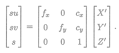
展开：



利用第3行消去(实际上就是 ${P}'$ 的距离)，得 $u=f_{x}\frac{{X}'}{{Z}'}+c_{x},v=f_{y}\frac{{Y}'}{{Z}'}+c_{y}$

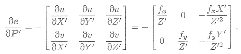
这与第5讲的相机模型是一致的。当我们求误差时，可以把这里的 $u,v$ 与实际的测量值比较，求差。在定义了中间变量后，我们对 $T$ 左乘扰动量 $\delta \xi$ ，然后考虑 $e$ 的变化关于扰动量的导数。利用链式法则，可以列写如下：

这里的 $\bigoplus$ 指李代数上的左乘扰动。第一项是误差关于投影点的导数，

易得

而第二项为变换后的点关于李代数的导数，根据4.3.2节中的推导，

得

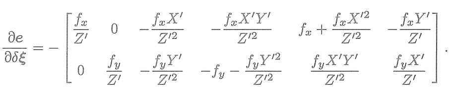
而在 ${P}'$ 的定义中，我们取出了前3维，于是得 $\frac{\partial {P}'}{\partial \delta \xi }=[I,-{P}'^{\wedge }]$

将这两项相乘，就得到了2×6的雅可比矩阵

这个雅可比矩阵描述了重投影误差关于相机位姿李代数的一阶变化关系。我们保留了前面的负号，这是因为误差是由观测值减预测值定义的。当然也可以反过来将它定义成“预测值减观测值”的形式。在那种情况下，只要去掉前面的负号即可。此外，如果 $se(3)$ 的定义方式是旋转在前，平移在后，则只要把这个矩阵的前3列与后3列对调即可。
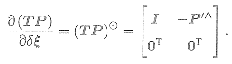
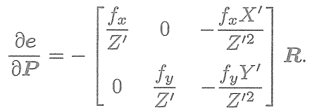
除了优化位姿，我们还希望优化特征点的空间位置。因此，需要讨论 $e$ 关于空间点 $P$ 的导数。利用链式法则，有 $\frac{\partial e}{\partial P }=\frac{\partial e}{\partial {P}' }\frac{\partial {P}'}{\partial P}$

第一项在前面已推导，关于第二项，按照定义 ${P}'=(TP)_{1:3}=RP+t$

我们发现 ${P}'$ 对 ${P}$ 求导后将只剩下 $R$ 。

于是



于是，我们推导出了观测相机方程关于相机位姿与特征点的两个导数矩阵。它们十分重要，能够在优化过程中提供重要的梯度方向，指导优化的迭代。

7.8 实践：求解PnP

7.8.1 使用EPnP求解位姿（调用OpenCV库）

首先，演示如何使用OpenCV的 EPnP求解PnP问题，然后通过非线性优化再次求解。由于PnP需要使用3D点，为了避免初始化带来的麻烦，使用RGB-D相机中的深度图( 1_depth.png)作为特征点的3D位置。

OpenCV提供的PnP函数如下：
int main(int argc, char **argv) {Mat r, t;solvePnP(pts_3d, pts_2d, K, Mat(), r, t, false); // 调用OpenCV 的 PnP 求解，可选择EPNP，DLS等方法Mat R;cout << "R=" << endl << R << endl;cout << "t=" << endl << t << endl;
在例程中，得到配对特征点后，在第一个图的深度图中寻找它们的深度，并求出空间位置。以此空间位置为3D点，再以第二个图像的像素位置为2D点，调用EPnP求解PnP问题。程序输出如下：
caohao@ubuntu:~/桌面/slam/slam_07/build$ ./pose_estimation_3d2d ../1.png ../2.png ../1_depth.png ../2_depth.png
-- Max dist : 95.000000 
-- Min dist : 4.000000 
一共找到了79组匹配点
3d-2d pairs: 76
solve pnp in opencv cost time: 0.0109459 seconds.
R=
[0.9978662025826269, -0.05167241613316376, 0.03991244360207524;0.0505958915956335, 0.998339762771668, 0.02752769192381471;-0.04126860182960625, -0.025449547736074, 0.998823919929363]
t=
[-0.1272259656955879;-0.007507297652615337;0.06138584177157709]
对比先前2D-2D情况下求解可以看到，在有3D信息时，估计的R几乎是相同的，而t相差得较多。这是由于引入了新的深度信息所致。不过，由于Kinect采集的深度图本身会有一些误差，所以这里的3D点也不是准确的。在较大规模的BA中，我们会希望把位姿和所有三维特征点同时优化。

7.8.2 手写位姿估计

演示如何使用非线性优化的方式计算相机位姿。先手写一个高斯牛顿法的PnP（高斯牛顿迭代优化），演示如何调用g2o来求解。

void bundleAdjustmentGaussNewton(const VecVector3d &points_3d,const VecVector2d &points_2d,const Mat &K,Sophus::SE3d &pose) {typedef Eigen::Matrix<double, 6, 1> Vector6d;const int iterations = 10;double cost = 0, lastCost = 0;double fx = K.at<double>(0, 0);double fy = K.at<double>(1, 1);double cx = K.at<double>(0, 2);double cy = K.at<double>(1, 2);for (int iter = 0; iter < iterations; iter++) {Eigen::Matrix<double, 6, 6> H = Eigen::Matrix<double, 6, 6>::Zero();Vector6d b = Vector6d::Zero();cost = 0;// compute costfor (int i = 0; i < points_3d.size(); i++) {Eigen::Vector3d pc = pose * points_3d[i];double inv_z = 1.0 / pc[2];double inv_z2 = inv_z * inv_z;Eigen::Vector2d proj(fx * pc[0] / pc[2] + cx, fy * pc[1] / pc[2] + cy);Eigen::Vector2d e = points_2d[i] - proj;cost += e.squaredNorm();Eigen::Matrix<double, 2, 6> J;J << -fx * inv_z,0,fx * pc[0] * inv_z2,fx * pc[0] * pc[1] * inv_z2,-fx - fx * pc[0] * pc[0] * inv_z2,fx * pc[1] * inv_z,0,-fy * inv_z,fy * pc[1] * inv_z2,fy + fy * pc[1] * pc[1] * inv_z2,-fy * pc[0] * pc[1] * inv_z2,-fy * pc[0] * inv_z;H += J.transpose() * J;b += -J.transpose() * e;}Vector6d dx;dx = H.ldlt().solve(b);if (isnan(dx[0])) {cout << "result is nan!" << endl;break;}if (iter > 0 && cost >= lastCost) {// cost increase, update is not goodcout << "cost: " << cost << ", last cost: " << lastCost << endl;break;}// update your estimationpose = Sophus::SE3d::exp(dx) * pose;lastCost = cost;cout << "iteration " << iter << " cost=" << std::setprecision(12) << cost << endl;if (dx.norm() < 1e-6) {// convergebreak;}}cout << "pose by g-n: \n" << pose.matrix() << endl;
}

7.8.3 使用g2o进行BA优化

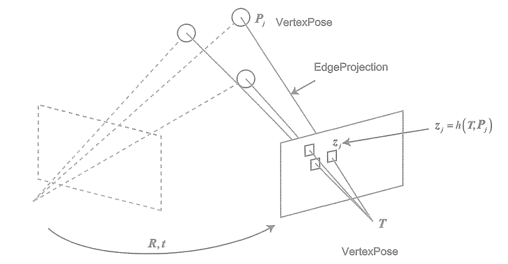
用g2o实现同样的操作（事实上，用Ceres 也完全类似)。g2o的基本知识见第6讲。在使用g2o之前，要把问题建模成一个图优化问题，如图。

在这个图优化中，节点和边的选择如下：

①节点：第二个相机的位姿节点T∈SE(3)。
②边：每个3D点在第二个相机中的投影，以观测方程来描述：

由于第一个相机位姿固定为零，所以没有把它写到优化变量里，但在更多的场合里，会考虑更多相机的估计。现在根据一组3D点和第二个图像中的2D投影，估计第二个相机的位姿。把第一个相机画成虚线表明不希望考虑它。
g2o提供了许多关于BA的节点和边，例如g2o/types/sba/types_six_dof_expmap.h中提供了李代数表达的节点和边。在本书中，我们自己实现一个 VertexPose顶点和EdgeProjection边，代码如下：

/// vertex and edges used in g2o ba
class VertexPose : public g2o::BaseVertex<6, Sophus::SE3d> {
public:EIGEN_MAKE_ALIGNED_OPERATOR_NEW;virtual void setToOriginImpl() override {_estimate = Sophus::SE3d();}/// left multiplication on SE3virtual void oplusImpl(const double *update) override {Eigen::Matrix<double, 6, 1> update_eigen;update_eigen << update[0], update[1], update[2], update[3], update[4], update[5];_estimate = Sophus::SE3d::exp(update_eigen) * _estimate;}virtual bool read(istream &in) override {}virtual bool write(ostream &out) const override {}
};class EdgeProjection : public g2o::BaseUnaryEdge<2, Eigen::Vector2d, VertexPose> {
public:EIGEN_MAKE_ALIGNED_OPERATOR_NEW;EdgeProjection(const Eigen::Vector3d &pos, const Eigen::Matrix3d &K) : _pos3d(pos), _K(K) {}virtual void computeError() override {const VertexPose *v = static_cast<VertexPose *> (_vertices[0]);Sophus::SE3d T = v->estimate();Eigen::Vector3d pos_pixel = _K * (T * _pos3d);pos_pixel /= pos_pixel[2];_error = _measurement - pos_pixel.head<2>();}virtual void linearizeOplus() override {const VertexPose *v = static_cast<VertexPose *> (_vertices[0]);Sophus::SE3d T = v->estimate();Eigen::Vector3d pos_cam = T * _pos3d;double fx = _K(0, 0);double fy = _K(1, 1);double cx = _K(0, 2);double cy = _K(1, 2);double X = pos_cam[0];double Y = pos_cam[1];double Z = pos_cam[2];double Z2 = Z * Z;_jacobianOplusXi<< -fx / Z, 0, fx * X / Z2, fx * X * Y / Z2, -fx - fx * X * X / Z2, fx * Y / Z,0, -fy / Z, fy * Y / (Z * Z), fy + fy * Y * Y / Z2, -fy * X * Y / Z2, -fy * X / Z;}virtual bool read(istream &in) override {}virtual bool write(ostream &out) const override {}private:Eigen::Vector3d _pos3d;Eigen::Matrix3d _K;
};

这里实现了顶点的更新和边的误差计算。下面将它们组成一个图优化问题：

void bundleAdjustmentG2O(const VecVector3d &points_3d,const VecVector2d &points_2d,const Mat &K,Sophus::SE3d &pose) {// 构建图优化，先设定g2otypedef g2o::BlockSolver<g2o::BlockSolverTraits<6, 3>> BlockSolverType;  // pose is 6, landmark is 3typedef g2o::LinearSolverDense<BlockSolverType::PoseMatrixType> LinearSolverType; // 线性求解器类型// 梯度下降方法，可以从GN, LM, DogLeg 中选auto solver = new g2o::OptimizationAlgorithmGaussNewton(g2o::make_unique<BlockSolverType>(g2o::make_unique<LinearSolverType>()));g2o::SparseOptimizer optimizer;     // 图模型optimizer.setAlgorithm(solver);   // 设置求解器optimizer.setVerbose(true);       // 打开调试输出// vertexVertexPose *vertex_pose = new VertexPose(); // camera vertex_posevertex_pose->setId(0);vertex_pose->setEstimate(Sophus::SE3d());optimizer.addVertex(vertex_pose);// KEigen::Matrix3d K_eigen;K_eigen <<K.at<double>(0, 0), K.at<double>(0, 1), K.at<double>(0, 2),K.at<double>(1, 0), K.at<double>(1, 1), K.at<double>(1, 2),K.at<double>(2, 0), K.at<double>(2, 1), K.at<double>(2, 2);// edgesint index = 1;for (size_t i = 0; i < points_2d.size(); ++i) {auto p2d = points_2d[i];auto p3d = points_3d[i];EdgeProjection *edge = new EdgeProjection(p3d, K_eigen);edge->setId(index);edge->setVertex(0, vertex_pose);edge->setMeasurement(p2d);edge->setInformation(Eigen::Matrix2d::Identity());optimizer.addEdge(edge);index++;}chrono::steady_clock::time_point t1 = chrono::steady_clock::now();optimizer.setVerbose(true);optimizer.initializeOptimization();optimizer.optimize(10);chrono::steady_clock::time_point t2 = chrono::steady_clock::now();chrono::duration<double> time_used = chrono::duration_cast<chrono::duration<double>>(t2 - t1);cout << "optimization costs time: " << time_used.count() << " seconds." << endl;cout << "pose estimated by g2o =\n" << vertex_pose->estimate().matrix() << endl;pose = vertex_pose->estimate();
}

程序大体上和第6讲的g2o类似。首先声明了g2o图优化器，并配置优化求解器和梯度下降方法。然后，根据估计到的特征点，将位姿和空间点放到图中。最后，调用优化函数进行求解。

（1）CmakeLists.txt

#声明要求cmake的最低版本
cmake_minimum_required(VERSION 3.16)#声明一个cmake工程
project(slam_07)set(CMAKE_CXX_STANDARD 17)
set(CMAKE_CXX_STANDARD_REQUIRED ON)
#启用最高优化级别，移除调试开销
set(CMAKE_BUILD_TYPE "Release")
#并行计算，加速运算
add_definitions("-DENABLE_SSE")
# 启用 SSE4.2 和 POPCNT 指令
set(CMAKE_CXX_FLAGS "${CMAKE_CXX_FLAGS} -msse4.2 -mpopcnt")list(APPEND CMAKE_MODULE_PATH ${PROJECT_SOURCE_DIR}/cmake)
list( APPEND CMAKE_MODULE_PATH /home/caohao/g2o/cmake_modules )# OpenCV
find_package(OpenCV 3 REQUIRED)
include_directories(${OpenCV_INCLUDE_DIRS})# g2o
find_package(G2O REQUIRED)
include_directories(${G2O_INCLUDE_DIRS})# Eigen
find_package(Eigen3 REQUIRED NO_MODULE)
include_directories("/usr/local/include/eigen3")
set(CMAKE_PREFIX_PATH "/usr/local" ${CMAKE_PREFIX_PATH})# 确保 Eigen3::Eigen target 存在
if(NOT TARGET Eigen3::Eigen)add_library(Eigen3::Eigen INTERFACE IMPORTED)set_target_properties(Eigen3::Eigen PROPERTIESINTERFACE_INCLUDE_DIRECTORIES "/usr/local/include/eigen3")
endif()# Sophus
set(EIGEN3_INCLUDE_DIR "/usr/local/include/eigen3")
include_directories(${EIGEN3_INCLUDE_DIR})find_package(Sophus REQUIRED NO_MODULE)
include_directories(${Sophus_INCLUDE_DIRS})# 添加一个可执行程序，可执行文件名 cpp文件名
add_executable(orb_cv orb_cv.cpp)
target_link_libraries(orb_cv ${OpenCV_LIBS})add_executable(orb_self orb_self.cpp)
target_link_libraries(orb_self ${OpenCV_LIBS})add_executable(pose_estimation_2d2d pose_estimation_2d2d.cpp)
target_link_libraries(pose_estimation_2d2d ${OpenCV_LIBS})add_executable(triangulation triangulation.cpp)
target_link_libraries(triangulation ${OpenCV_LIBS})add_executable(pose_estimation_3d2d pose_estimation_3d2d.cpp)
target_link_libraries(pose_estimation_3d2d ${OpenCV_LIBS} g2o_core g2o_stuffSophus::Sophus
)

（2）程序代码pose_estimation_3d2d.cpp

#include <iostream>
#include <opencv2/core/core.hpp>
#include <opencv2/features2d/features2d.hpp>
#include <opencv2/highgui/highgui.hpp>
#include <opencv2/calib3d/calib3d.hpp>
#include <Eigen/Core>
#include <g2o/core/base_vertex.h>
#include <g2o/core/base_unary_edge.h>
#include <g2o/core/sparse_optimizer.h>
#include <g2o/core/block_solver.h>
#include <g2o/core/solver.h>
#include <g2o/core/optimization_algorithm_gauss_newton.h>
#include <g2o/solvers/dense/linear_solver_dense.h>
#include <sophus/se3.hpp>
#include <chrono>using namespace std;
using namespace cv;void find_feature_matches(const Mat &img_1, const Mat &img_2,std::vector<KeyPoint> &keypoints_1,std::vector<KeyPoint> &keypoints_2,std::vector<DMatch> &matches);// 像素坐标转相机归一化坐标
Point2d pixel2cam(const Point2d &p, const Mat &K);// BA by g2o
typedef vector<Eigen::Vector2d, Eigen::aligned_allocator<Eigen::Vector2d>> VecVector2d;
typedef vector<Eigen::Vector3d, Eigen::aligned_allocator<Eigen::Vector3d>> VecVector3d;void bundleAdjustmentG2O(const VecVector3d &points_3d,const VecVector2d &points_2d,const Mat &K,Sophus::SE3d &pose
);// BA by gauss-newton
void bundleAdjustmentGaussNewton(const VecVector3d &points_3d,const VecVector2d &points_2d,const Mat &K,Sophus::SE3d &pose
);int main(int argc, char **argv) {if (argc != 5) {cout << "usage: pose_estimation_3d2d img1 img2 depth1 depth2" << endl;return 1;}//-- 读取图像Mat img_1 = imread("../1.png");Mat img_2 = imread("../2.png");assert(img_1.data && img_2.data && "Can not load images!");vector<KeyPoint> keypoints_1, keypoints_2;vector<DMatch> matches;find_feature_matches(img_1, img_2, keypoints_1, keypoints_2, matches);cout << "一共找到了" << matches.size() << "组匹配点" << endl;// 建立3D点Mat d1 = imread(argv[3], CV_LOAD_IMAGE_UNCHANGED);       // 深度图为16位无符号数，单通道图像Mat K = (Mat_<double>(3, 3) << 520.9, 0, 325.1, 0, 521.0, 249.7, 0, 0, 1);vector<Point3f> pts_3d;vector<Point2f> pts_2d;for (DMatch m:matches) {ushort d = d1.ptr<unsigned short>(int(keypoints_1[m.queryIdx].pt.y))[int(keypoints_1[m.queryIdx].pt.x)];if (d == 0)   // bad depthcontinue;float dd = d / 5000.0;Point2d p1 = pixel2cam(keypoints_1[m.queryIdx].pt, K);pts_3d.push_back(Point3f(p1.x * dd, p1.y * dd, dd));pts_2d.push_back(keypoints_2[m.trainIdx].pt);}cout << "3d-2d pairs: " << pts_3d.size() << endl;chrono::steady_clock::time_point t1 = chrono::steady_clock::now();Mat r, t;solvePnP(pts_3d, pts_2d, K, Mat(), r, t, false); // 调用OpenCV 的 PnP 求解，可选择EPNP，DLS等方法Mat R;cv::Rodrigues(r, R); // r为旋转向量形式，用Rodrigues公式转换为矩阵chrono::steady_clock::time_point t2 = chrono::steady_clock::now();chrono::duration<double> time_used = chrono::duration_cast<chrono::duration<double>>(t2 - t1);cout << "solve pnp in opencv cost time: " << time_used.count() << " seconds." << endl;cout << "R=" << endl << R << endl;cout << "t=" << endl << t << endl;VecVector3d pts_3d_eigen;VecVector2d pts_2d_eigen;for (size_t i = 0; i < pts_3d.size(); ++i) {pts_3d_eigen.push_back(Eigen::Vector3d(pts_3d[i].x, pts_3d[i].y, pts_3d[i].z));pts_2d_eigen.push_back(Eigen::Vector2d(pts_2d[i].x, pts_2d[i].y));}cout << "calling bundle adjustment by gauss newton" << endl;Sophus::SE3d pose_gn;t1 = chrono::steady_clock::now();bundleAdjustmentGaussNewton(pts_3d_eigen, pts_2d_eigen, K, pose_gn);t2 = chrono::steady_clock::now();time_used = chrono::duration_cast<chrono::duration<double>>(t2 - t1);cout << "solve pnp by gauss newton cost time: " << time_used.count() << " seconds." << endl;cout << "calling bundle adjustment by g2o" << endl;Sophus::SE3d pose_g2o;t1 = chrono::steady_clock::now();bundleAdjustmentG2O(pts_3d_eigen, pts_2d_eigen, K, pose_g2o);t2 = chrono::steady_clock::now();time_used = chrono::duration_cast<chrono::duration<double>>(t2 - t1);cout << "solve pnp by g2o cost time: " << time_used.count() << " seconds." << endl;return 0;
}void find_feature_matches(const Mat &img_1, const Mat &img_2,std::vector<KeyPoint> &keypoints_1,std::vector<KeyPoint> &keypoints_2,std::vector<DMatch> &matches) {//-- 初始化Mat descriptors_1, descriptors_2;// used in OpenCV3Ptr<FeatureDetector> detector = ORB::create();Ptr<DescriptorExtractor> descriptor = ORB::create();// use this if you are in OpenCV2// Ptr<FeatureDetector> detector = FeatureDetector::create ( "ORB" );// Ptr<DescriptorExtractor> descriptor = DescriptorExtractor::create ( "ORB" );Ptr<DescriptorMatcher> matcher = DescriptorMatcher::create("BruteForce-Hamming");//-- 第一步:检测 Oriented FAST 角点位置detector->detect(img_1, keypoints_1);detector->detect(img_2, keypoints_2);//-- 第二步:根据角点位置计算 BRIEF 描述子descriptor->compute(img_1, keypoints_1, descriptors_1);descriptor->compute(img_2, keypoints_2, descriptors_2);//-- 第三步:对两幅图像中的BRIEF描述子进行匹配，使用 Hamming 距离vector<DMatch> match;// BFMatcher matcher ( NORM_HAMMING );matcher->match(descriptors_1, descriptors_2, match);//-- 第四步:匹配点对筛选double min_dist = 10000, max_dist = 0;//找出所有匹配之间的最小距离和最大距离, 即是最相似的和最不相似的两组点之间的距离for (int i = 0; i < descriptors_1.rows; i++) {double dist = match[i].distance;if (dist < min_dist) min_dist = dist;if (dist > max_dist) max_dist = dist;}printf("-- Max dist : %f \n", max_dist);printf("-- Min dist : %f \n", min_dist);//当描述子之间的距离大于两倍的最小距离时,即认为匹配有误.但有时候最小距离会非常小,设置一个经验值30作为下限.for (int i = 0; i < descriptors_1.rows; i++) {if (match[i].distance <= max(2 * min_dist, 30.0)) {matches.push_back(match[i]);}}
}Point2d pixel2cam(const Point2d &p, const Mat &K) {return Point2d((p.x - K.at<double>(0, 2)) / K.at<double>(0, 0),(p.y - K.at<double>(1, 2)) / K.at<double>(1, 1));
}void bundleAdjustmentGaussNewton(const VecVector3d &points_3d,const VecVector2d &points_2d,const Mat &K,Sophus::SE3d &pose) {typedef Eigen::Matrix<double, 6, 1> Vector6d;const int iterations = 10;double cost = 0, lastCost = 0;double fx = K.at<double>(0, 0);double fy = K.at<double>(1, 1);double cx = K.at<double>(0, 2);double cy = K.at<double>(1, 2);for (int iter = 0; iter < iterations; iter++) {Eigen::Matrix<double, 6, 6> H = Eigen::Matrix<double, 6, 6>::Zero();Vector6d b = Vector6d::Zero();cost = 0;// compute costfor (int i = 0; i < points_3d.size(); i++) {Eigen::Vector3d pc = pose * points_3d[i];double inv_z = 1.0 / pc[2];double inv_z2 = inv_z * inv_z;Eigen::Vector2d proj(fx * pc[0] / pc[2] + cx, fy * pc[1] / pc[2] + cy);Eigen::Vector2d e = points_2d[i] - proj;cost += e.squaredNorm();Eigen::Matrix<double, 2, 6> J;J << -fx * inv_z,0,fx * pc[0] * inv_z2,fx * pc[0] * pc[1] * inv_z2,-fx - fx * pc[0] * pc[0] * inv_z2,fx * pc[1] * inv_z,0,-fy * inv_z,fy * pc[1] * inv_z2,fy + fy * pc[1] * pc[1] * inv_z2,-fy * pc[0] * pc[1] * inv_z2,-fy * pc[0] * inv_z;H += J.transpose() * J;b += -J.transpose() * e;}Vector6d dx;dx = H.ldlt().solve(b);if (isnan(dx[0])) {cout << "result is nan!" << endl;break;}if (iter > 0 && cost >= lastCost) {// cost increase, update is not goodcout << "cost: " << cost << ", last cost: " << lastCost << endl;break;}// update your estimationpose = Sophus::SE3d::exp(dx) * pose;lastCost = cost;cout << "iteration " << iter << " cost=" << std::setprecision(12) << cost << endl;if (dx.norm() < 1e-6) {// convergebreak;}}cout << "pose by g-n: \n" << pose.matrix() << endl;
}/// vertex and edges used in g2o ba
class VertexPose : public g2o::BaseVertex<6, Sophus::SE3d> {
public:EIGEN_MAKE_ALIGNED_OPERATOR_NEW;virtual void setToOriginImpl() override {_estimate = Sophus::SE3d();}/// left multiplication on SE3virtual void oplusImpl(const double *update) override {Eigen::Matrix<double, 6, 1> update_eigen;update_eigen << update[0], update[1], update[2], update[3], update[4], update[5];_estimate = Sophus::SE3d::exp(update_eigen) * _estimate;}virtual bool read(istream &in) override {}virtual bool write(ostream &out) const override {}
};class EdgeProjection : public g2o::BaseUnaryEdge<2, Eigen::Vector2d, VertexPose> {
public:EIGEN_MAKE_ALIGNED_OPERATOR_NEW;EdgeProjection(const Eigen::Vector3d &pos, const Eigen::Matrix3d &K) : _pos3d(pos), _K(K) {}virtual void computeError() override {const VertexPose *v = static_cast<VertexPose *> (_vertices[0]);Sophus::SE3d T = v->estimate();Eigen::Vector3d pos_pixel = _K * (T * _pos3d);pos_pixel /= pos_pixel[2];_error = _measurement - pos_pixel.head<2>();}virtual void linearizeOplus() override {const VertexPose *v = static_cast<VertexPose *> (_vertices[0]);Sophus::SE3d T = v->estimate();Eigen::Vector3d pos_cam = T * _pos3d;double fx = _K(0, 0);double fy = _K(1, 1);double cx = _K(0, 2);double cy = _K(1, 2);double X = pos_cam[0];double Y = pos_cam[1];double Z = pos_cam[2];double Z2 = Z * Z;_jacobianOplusXi<< -fx / Z, 0, fx * X / Z2, fx * X * Y / Z2, -fx - fx * X * X / Z2, fx * Y / Z,0, -fy / Z, fy * Y / (Z * Z), fy + fy * Y * Y / Z2, -fy * X * Y / Z2, -fy * X / Z;}virtual bool read(istream &in) override {}virtual bool write(ostream &out) const override {}private:Eigen::Vector3d _pos3d;Eigen::Matrix3d _K;
};void bundleAdjustmentG2O(const VecVector3d &points_3d,const VecVector2d &points_2d,const Mat &K,Sophus::SE3d &pose) {// 构建图优化，先设定g2otypedef g2o::BlockSolver<g2o::BlockSolverTraits<6, 3>> BlockSolverType;  // pose is 6, landmark is 3typedef g2o::LinearSolverDense<BlockSolverType::PoseMatrixType> LinearSolverType; // 线性求解器类型// 梯度下降方法，可以从GN, LM, DogLeg 中选auto solver = new g2o::OptimizationAlgorithmGaussNewton(g2o::make_unique<BlockSolverType>(g2o::make_unique<LinearSolverType>()));g2o::SparseOptimizer optimizer;     // 图模型optimizer.setAlgorithm(solver);   // 设置求解器optimizer.setVerbose(true);       // 打开调试输出// vertexVertexPose *vertex_pose = new VertexPose(); // camera vertex_posevertex_pose->setId(0);vertex_pose->setEstimate(Sophus::SE3d());optimizer.addVertex(vertex_pose);// KEigen::Matrix3d K_eigen;K_eigen <<K.at<double>(0, 0), K.at<double>(0, 1), K.at<double>(0, 2),K.at<double>(1, 0), K.at<double>(1, 1), K.at<double>(1, 2),K.at<double>(2, 0), K.at<double>(2, 1), K.at<double>(2, 2);// edgesint index = 1;for (size_t i = 0; i < points_2d.size(); ++i) {auto p2d = points_2d[i];auto p3d = points_3d[i];EdgeProjection *edge = new EdgeProjection(p3d, K_eigen);edge->setId(index);edge->setVertex(0, vertex_pose);edge->setMeasurement(p2d);edge->setInformation(Eigen::Matrix2d::Identity());optimizer.addEdge(edge);index++;}chrono::steady_clock::time_point t1 = chrono::steady_clock::now();optimizer.setVerbose(true);optimizer.initializeOptimization();optimizer.optimize(10);chrono::steady_clock::time_point t2 = chrono::steady_clock::now();chrono::duration<double> time_used = chrono::duration_cast<chrono::duration<double>>(t2 - t1);cout << "optimization costs time: " << time_used.count() << " seconds." << endl;cout << "pose estimated by g2o =\n" << vertex_pose->estimate().matrix() << endl;pose = vertex_pose->estimate();
}

（3）运行的输出如下：

caohao@ubuntu:~/桌面/slam/slam_07/build$ ./pose_estimation_3d2d ../1.png ../2.png ../1_depth.png ../2_depth.png
-- Max dist : 95.000000 
-- Min dist : 4.000000 
一共找到了79组匹配点
3d-2d pairs: 76
solve pnp in opencv cost time: 0.0109459 seconds.
R=
[0.9978662025826269, -0.05167241613316376, 0.03991244360207524;0.0505958915956335, 0.998339762771668, 0.02752769192381471;-0.04126860182960625, -0.025449547736074, 0.998823919929363]
t=
[-0.1272259656955879;-0.007507297652615337;0.06138584177157709]
calling bundle adjustment by gauss newton
iteration 0 cost=45538.1857253
iteration 1 cost=413.221881688
iteration 2 cost=301.36705717
iteration 3 cost=301.365779441
pose by g-n: 0.99786620258  -0.0516724160901   0.0399124437155   -0.1272259658860.050595891549    0.998339762774     0.02752769194 -0.00750729768072-0.0412686019426  -0.0254495477483    0.998823919924   0.06138584181510                 0                 0                 1
solve pnp by gauss newton cost time: 0.000261044 seconds.
calling bundle adjustment by g2o
iteration= 0	 chi2= 413.221882	 time= 3.1152e-05	 cumTime= 3.1152e-05	 edges= 76	 schur= 0
iteration= 1	 chi2= 301.367057	 time= 1.45281e-05	 cumTime= 4.56801e-05	 edges= 76	 schur= 0
iteration= 2	 chi2= 301.365779	 time= 1.8e-05	 cumTime= 6.36801e-05	 edges= 76	 schur= 0
iteration= 3	 chi2= 301.365779	 time= 1.61299e-05	 cumTime= 7.981e-05	 edges= 76	 schur= 0
iteration= 4	 chi2= 301.365779	 time= 1.42941e-05	 cumTime= 9.41041e-05	 edges= 76	 schur= 0
iteration= 5	 chi2= 301.365779	 time= 1.4359e-05	 cumTime= 0.000108463	 edges= 76	 schur= 0
iteration= 6	 chi2= 301.365779	 time= 1.48481e-05	 cumTime= 0.000123311	 edges= 76	 schur= 0
iteration= 7	 chi2= 301.365779	 time= 1.3574e-05	 cumTime= 0.000136885	 edges= 76	 schur= 0
iteration= 8	 chi2= 301.365779	 time= 1.7683e-05	 cumTime= 0.000154568	 edges= 76	 schur= 0
iteration= 9	 chi2= 301.365779	 time= 1.4461e-05	 cumTime= 0.000169029	 edges= 76	 schur= 0
optimization costs time: 0.000962538 seconds.
pose estimated by g2o =0.997866202583  -0.0516724161336   0.0399124436024   -0.1272259656960.050595891596    0.998339762772   0.0275276919261 -0.00750729765631-0.04126860183  -0.0254495477384    0.998823919929   0.06138584177110                 0                 0                 1
solve pnp by g2o cost time: 0.003256208 seconds.

从估计结果上看，三者基本一致。从优化时间来看，实现的高斯牛顿法排在第一，其次是OpenCV的PnP，最后是g2o的实现。尽管如此，三者的用时都在1毫秒以内，这说明位姿估计算法并不耗费计算量。
BA是一种通用的做法。它可以不限于两幅图像。完全可以放入多幅图像匹配到的位姿和空间点进行迭代优化，甚至可以把整个SLAM过程放进来。那种做法规模较大，主要在后端使用，第10讲会再次遇到这个问题。在前端，通常考虑局部相机位姿和特征点的小型BA问题，希望对它进行实时求解和优化。

7.8.4 报错修复

1.报错代码

caohao@ubuntu:~/桌面/slam/slam_07/build$ ./pose_estimation_3d2d ../1.png ../2.png ../1_depth.png ../2_depth.png
-- Max dist : 0.000000 
-- Min dist : 10000.000000 
一共找到了0组匹配点
3d-2d pairs: 0
OpenCV Error: Assertion failed (npoints >= 0 && npoints == std::max(ipoints.checkVector(2, CV_32F), ipoints.checkVector(2, CV_64F))) in solvePnP, file /build/opencv-L2vuMj/opencv-3.2.0+dfsg/modules/calib3d/src/solvepnp.cpp, line 63
terminate called after throwing an instance of 'cv::Exception'what():  /build/opencv-L2vuMj/opencv-3.2.0+dfsg/modules/calib3d/src/solvepnp.cpp:63: error: (-215) npoints >= 0 && npoints == std::max(ipoints.checkVector(2, CV_32F), ipoints.checkVector(2, CV_64F)) in function solvePnP已放弃 (核心已转储)

2.检查与修复

（1）检查Eigen3是否安装，笔者版本3.4

（2）确认Eigen3.4安装位置，笔者/usr/local/include/eigen3/Eigen

（3）确认是否有SophusConfig.cmake，查找路径/usr/local/share/sophus/cmake/SophusConfig.cmake

（4）如上述都有修改CmakeLists.txt（如上），编译是运行如下指令
cd ~/桌面/slam/slam_07/build
rm -rf *
cmake .. -DEigen3_INCLUDE_DIR=/usr/local/include/eigen3
make -j4

7.9 3D-3D：ICP

假设有一组配对好的3D点(例如我们对两幅RGB-D图像进行了匹配)：

$P=\left \{ p_{1},...,p_{n} \right \},P^{'}=\left \{ p_{1}^{'},...,p_{n}^{'} \right \}$

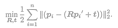
现在，想要找一个欧氏变换，使得 $\forall i,p_{'}=R p_{i}^{'}+t$

这个问题可以用迭代最近点(Iterative Closest Point,ICP)求解。

3D-3D位姿估计问题中并没有出现相机模型，仅考虑两组3D点之间的变换时和相机无关。因此，在激光SLAM中也会碰到ICP，不过由于激光数据特征不够丰富，无从知道两个点集之间的匹配关系，只能认为距离最近的两个点为同一个。
所以这个方法称为迭代最近点。而在视觉中，特征点为我们提供了较好的匹配关系，所以整个问题就变得更简单了。在RGB-D SLAM中，可以用这种方式估计相机位姿。下文我们用ICP指代匹配好的两组点间的运动估计问题。
和 PnP类似，ICP的求解也分为两种方式：利用线性代数的求解(主要是SVD)，以及利用非线性优化方式的求解(类似于BA)。

7.9.1 SVD法（线性代数求解）

定义第i对点的误差项： $e_{i}=p_{i}-(Rp_{i}^{'}+t)$
构建最小二乘问题，求使误差平方和达到极小的R、t（公式推导略）：

ICP可以分为以下三个步骤求解：

①计算两组点的质心位置 $p,p_{i}$ ，然后计算每个点的去质心坐标： $q_{i}=p_{i}-p,q_{i}^{'}=p_{i}^{'}-p^{'}$

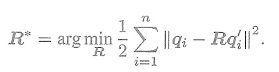
②根据以下优化问题计算旋转矩阵：

③根据第2步的R计算t： $t^{*}=p-Rp_{i}$

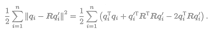
我们看到,只要求出了两组点之间的旋转，平移量是非常容易得到的。所以重点关注R的计算。展开关于R的误差项，得

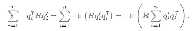
注意到第一项和R无关，第二项由于 $R^{T}R=I$ ，亦与R无关。因此，实际上优化目标函
数变为

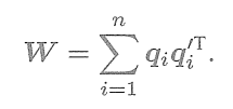
接下来通过SVD解出上述问题中最优的R。为了解R，先定义矩阵

W是一个3×3的矩阵，对W进行SVD分解，得 $W=U\sum V^{T}$

其中， $\sum$ 为奇异值组成的对角矩阵，对角线元素从大到小排列，U,V为对角矩阵。当W满秩时，R为 $R=UV^{T}$

解得R后，求解t即可。如果此时R的行列式为负，则取-R作为最优值。

7.9.2 非线性优化方法

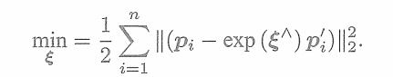
非线性优化方法是以迭代的方式去找最优值。该方法和 PnP非常相似。以李代数表达位姿时，目标函数写成

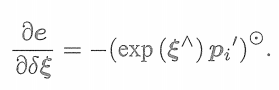
单个误差项关于位姿的导数在前面已推导，使用李代数扰动模型

于是，在非线性优化中只需不断迭代，就能找到极小值。而且，可以证明，ICP问题存在
唯一解或无穷多解的情况。在唯一解的情况下，只要能找到极小值解，这个极小值就是全局最优值——因此不会遇到局部极小而非全局最小的情况。这也意味着ICP求解可以任意选定初始值。这是已匹配点时求解ICP的一大好处。
这里讲的ICP是指已由图像特征给定了匹配的情况下进行位姿估计的问题。在匹配已知的情况下，这个最小二乘问题实际上具有解析解，所以并没有必要进行迭代优化。ICP的研究者们往往更加关心匹配未知的情况。那么，为什么我们要介绍基于优化的ICP呢？这是因为，某些场合下，例如在RGB-D SLAM中，一个像素的深度数据可能有，也可能测量不到，所以我们可以混合着使用PnP和ICP优化：对于深度已知的特征点，建模它们的3D-3D误差；对于深度未知的特征点，则建模3D-2D的重投影误差。于是，可以将所有的误差放在同一个问题中考虑,使得求解更加方便。

7.10 实践：求解ICP

7.10.1 实践：SVD方法

使用SVD及非线性优化来求解ICP。本节使用两幅RGB-D图像，通过特征匹配获取两组3D点，最后用ICP计算它们的位姿变换。由于OpenCV目前还没有计算两组带匹配点的ICP的方法，而且它的原理也并不复杂，所以我们自己来实现一个ICP。

1.pose_estimation_3d3d.cpp

#include <iostream>
#include <opencv2/core/core.hpp>
#include <opencv2/features2d/features2d.hpp>
#include <opencv2/highgui/highgui.hpp>
#include <opencv2/calib3d/calib3d.hpp>
#include <Eigen/Core>
#include <Eigen/Dense>
#include <Eigen/Geometry>
#include <Eigen/SVD>
#include <g2o/core/base_vertex.h>
#include <g2o/core/base_unary_edge.h>
#include <g2o/core/block_solver.h>
#include <g2o/core/optimization_algorithm_gauss_newton.h>
#include <g2o/core/optimization_algorithm_levenberg.h>
#include <g2o/solvers/dense/linear_solver_dense.h>
#include <chrono>
#include <sophus/se3.hpp>using namespace std;
using namespace cv;void find_feature_matches(const Mat &img_1, const Mat &img_2,std::vector<KeyPoint> &keypoints_1,std::vector<KeyPoint> &keypoints_2,std::vector<DMatch> &matches);// 像素坐标转相机归一化坐标
Point2d pixel2cam(const Point2d &p, const Mat &K);void pose_estimation_3d3d(const vector<Point3f> &pts1,const vector<Point3f> &pts2,Mat &R, Mat &t
);void bundleAdjustment(const vector<Point3f> &points_3d,const vector<Point3f> &points_2d,Mat &R, Mat &t
);/// vertex and edges used in g2o ba
class VertexPose : public g2o::BaseVertex<6, Sophus::SE3d> {
public:EIGEN_MAKE_ALIGNED_OPERATOR_NEW;virtual void setToOriginImpl() override {_estimate = Sophus::SE3d();}/// left multiplication on SE3virtual void oplusImpl(const double *update) override {Eigen::Matrix<double, 6, 1> update_eigen;update_eigen << update[0], update[1], update[2], update[3], update[4], update[5];_estimate = Sophus::SE3d::exp(update_eigen) * _estimate;}virtual bool read(istream &in) override {}virtual bool write(ostream &out) const override {}
};/// g2o edge
class EdgeProjectXYZRGBDPoseOnly : public g2o::BaseUnaryEdge<3, Eigen::Vector3d, VertexPose> {
public:EIGEN_MAKE_ALIGNED_OPERATOR_NEW;EdgeProjectXYZRGBDPoseOnly(const Eigen::Vector3d &point) : _point(point) {}virtual void computeError() override {const VertexPose *pose = static_cast<const VertexPose *> ( _vertices[0] );_error = _measurement - pose->estimate() * _point;}virtual void linearizeOplus() override {VertexPose *pose = static_cast<VertexPose *>(_vertices[0]);Sophus::SE3d T = pose->estimate();Eigen::Vector3d xyz_trans = T * _point;_jacobianOplusXi.block<3, 3>(0, 0) = -Eigen::Matrix3d::Identity();_jacobianOplusXi.block<3, 3>(0, 3) = Sophus::SO3d::hat(xyz_trans);}bool read(istream &in) {}bool write(ostream &out) const {}protected:Eigen::Vector3d _point;
};int main(int argc, char **argv) {if (argc != 5) {cout << "usage: pose_estimation_3d3d img1 img2 depth1 depth2" << endl;return 1;}//-- 读取图像Mat img_1 = imread("../1.png");Mat img_2 = imread("../2.png");vector<KeyPoint> keypoints_1, keypoints_2;vector<DMatch> matches;find_feature_matches(img_1, img_2, keypoints_1, keypoints_2, matches);cout << "一共找到了" << matches.size() << "组匹配点" << endl;// 建立3D点Mat depth1 = imread(argv[3], CV_LOAD_IMAGE_UNCHANGED);       // 深度图为16位无符号数，单通道图像Mat depth2 = imread(argv[4], CV_LOAD_IMAGE_UNCHANGED);       // 深度图为16位无符号数，单通道图像Mat K = (Mat_<double>(3, 3) << 520.9, 0, 325.1, 0, 521.0, 249.7, 0, 0, 1);vector<Point3f> pts1, pts2;for (DMatch m:matches) {ushort d1 = depth1.ptr<unsigned short>(int(keypoints_1[m.queryIdx].pt.y))[int(keypoints_1[m.queryIdx].pt.x)];ushort d2 = depth2.ptr<unsigned short>(int(keypoints_2[m.trainIdx].pt.y))[int(keypoints_2[m.trainIdx].pt.x)];if (d1 == 0 || d2 == 0)   // bad depthcontinue;Point2d p1 = pixel2cam(keypoints_1[m.queryIdx].pt, K);Point2d p2 = pixel2cam(keypoints_2[m.trainIdx].pt, K);float dd1 = float(d1) / 5000.0;float dd2 = float(d2) / 5000.0;pts1.push_back(Point3f(p1.x * dd1, p1.y * dd1, dd1));pts2.push_back(Point3f(p2.x * dd2, p2.y * dd2, dd2));}cout << "3d-3d pairs: " << pts1.size() << endl;Mat R, t;pose_estimation_3d3d(pts1, pts2, R, t);cout << "ICP via SVD results: " << endl;cout << "R = " << R << endl;cout << "t = " << t << endl;cout << "R_inv = " << R.t() << endl;cout << "t_inv = " << -R.t() * t << endl;cout << "calling bundle adjustment" << endl;bundleAdjustment(pts1, pts2, R, t);// verify p1 = R * p2 + tfor (int i = 0; i < 5; i++) {cout << "p1 = " << pts1[i] << endl;cout << "p2 = " << pts2[i] << endl;cout << "(R*p2+t) = " <<R * (Mat_<double>(3, 1) << pts2[i].x, pts2[i].y, pts2[i].z) + t<< endl;cout << endl;}
}void find_feature_matches(const Mat &img_1, const Mat &img_2,std::vector<KeyPoint> &keypoints_1,std::vector<KeyPoint> &keypoints_2,std::vector<DMatch> &matches) {//-- 初始化Mat descriptors_1, descriptors_2;// used in OpenCV3Ptr<FeatureDetector> detector = ORB::create();Ptr<DescriptorExtractor> descriptor = ORB::create();// use this if you are in OpenCV2// Ptr<FeatureDetector> detector = FeatureDetector::create ( "ORB" );// Ptr<DescriptorExtractor> descriptor = DescriptorExtractor::create ( "ORB" );Ptr<DescriptorMatcher> matcher = DescriptorMatcher::create("BruteForce-Hamming");//-- 第一步:检测 Oriented FAST 角点位置detector->detect(img_1, keypoints_1);detector->detect(img_2, keypoints_2);//-- 第二步:根据角点位置计算 BRIEF 描述子descriptor->compute(img_1, keypoints_1, descriptors_1);descriptor->compute(img_2, keypoints_2, descriptors_2);//-- 第三步:对两幅图像中的BRIEF描述子进行匹配，使用 Hamming 距离vector<DMatch> match;// BFMatcher matcher ( NORM_HAMMING );matcher->match(descriptors_1, descriptors_2, match);//-- 第四步:匹配点对筛选double min_dist = 10000, max_dist = 0;//找出所有匹配之间的最小距离和最大距离, 即是最相似的和最不相似的两组点之间的距离for (int i = 0; i < descriptors_1.rows; i++) {double dist = match[i].distance;if (dist < min_dist) min_dist = dist;if (dist > max_dist) max_dist = dist;}printf("-- Max dist : %f \n", max_dist);printf("-- Min dist : %f \n", min_dist);//当描述子之间的距离大于两倍的最小距离时,即认为匹配有误.但有时候最小距离会非常小,设置一个经验值30作为下限.for (int i = 0; i < descriptors_1.rows; i++) {if (match[i].distance <= max(2 * min_dist, 30.0)) {matches.push_back(match[i]);}}
}Point2d pixel2cam(const Point2d &p, const Mat &K) {return Point2d((p.x - K.at<double>(0, 2)) / K.at<double>(0, 0),(p.y - K.at<double>(1, 2)) / K.at<double>(1, 1));
}void pose_estimation_3d3d(const vector<Point3f> &pts1,const vector<Point3f> &pts2,Mat &R, Mat &t) {Point3f p1, p2;     // center of massint N = pts1.size();for (int i = 0; i < N; i++) {p1 += pts1[i];p2 += pts2[i];}p1 = Point3f(Vec3f(p1) / N);p2 = Point3f(Vec3f(p2) / N);vector<Point3f> q1(N), q2(N); // remove the centerfor (int i = 0; i < N; i++) {q1[i] = pts1[i] - p1;q2[i] = pts2[i] - p2;}// compute q1*q2^TEigen::Matrix3d W = Eigen::Matrix3d::Zero();for (int i = 0; i < N; i++) {W += Eigen::Vector3d(q1[i].x, q1[i].y, q1[i].z) * Eigen::Vector3d(q2[i].x, q2[i].y, q2[i].z).transpose();}cout << "W=" << W << endl;// SVD on WEigen::JacobiSVD<Eigen::Matrix3d> svd(W, Eigen::ComputeFullU | Eigen::ComputeFullV);Eigen::Matrix3d U = svd.matrixU();Eigen::Matrix3d V = svd.matrixV();cout << "U=" << U << endl;cout << "V=" << V << endl;Eigen::Matrix3d R_ = U * (V.transpose());if (R_.determinant() < 0) {R_ = -R_;}Eigen::Vector3d t_ = Eigen::Vector3d(p1.x, p1.y, p1.z) - R_ * Eigen::Vector3d(p2.x, p2.y, p2.z);// convert to cv::MatR = (Mat_<double>(3, 3) <<R_(0, 0), R_(0, 1), R_(0, 2),R_(1, 0), R_(1, 1), R_(1, 2),R_(2, 0), R_(2, 1), R_(2, 2));t = (Mat_<double>(3, 1) << t_(0, 0), t_(1, 0), t_(2, 0));
}void bundleAdjustment(const vector<Point3f> &pts1,const vector<Point3f> &pts2,Mat &R, Mat &t) {// 构建图优化，先设定g2otypedef g2o::BlockSolverX BlockSolverType;typedef g2o::LinearSolverDense<BlockSolverType::PoseMatrixType> LinearSolverType; // 线性求解器类型// 梯度下降方法，可以从GN, LM, DogLeg 中选auto solver = new g2o::OptimizationAlgorithmLevenberg(g2o::make_unique<BlockSolverType>(g2o::make_unique<LinearSolverType>()));g2o::SparseOptimizer optimizer;     // 图模型optimizer.setAlgorithm(solver);   // 设置求解器optimizer.setVerbose(true);       // 打开调试输出// vertexVertexPose *pose = new VertexPose(); // camera posepose->setId(0);pose->setEstimate(Sophus::SE3d());optimizer.addVertex(pose);// edgesfor (size_t i = 0; i < pts1.size(); i++) {EdgeProjectXYZRGBDPoseOnly *edge = new EdgeProjectXYZRGBDPoseOnly(Eigen::Vector3d(pts2[i].x, pts2[i].y, pts2[i].z));edge->setVertex(0, pose);edge->setMeasurement(Eigen::Vector3d(pts1[i].x, pts1[i].y, pts1[i].z));edge->setInformation(Eigen::Matrix3d::Identity());optimizer.addEdge(edge);}chrono::steady_clock::time_point t1 = chrono::steady_clock::now();optimizer.initializeOptimization();optimizer.optimize(10);chrono::steady_clock::time_point t2 = chrono::steady_clock::now();chrono::duration<double> time_used = chrono::duration_cast<chrono::duration<double>>(t2 - t1);cout << "optimization costs time: " << time_used.count() << " seconds." << endl;cout << endl << "after optimization:" << endl;cout << "T=\n" << pose->estimate().matrix() << endl;// convert to cv::MatEigen::Matrix3d R_ = pose->estimate().rotationMatrix();Eigen::Vector3d t_ = pose->estimate().translation();R = (Mat_<double>(3, 3) <<R_(0, 0), R_(0, 1), R_(0, 2),R_(1, 0), R_(1, 1), R_(1, 2),R_(2, 0), R_(2, 1), R_(2, 2));t = (Mat_<double>(3, 1) << t_(0, 0), t_(1, 0), t_(2, 0));
}

2.CmakeLists.txt

#include_directories("/usr/include/eigen3")
include_directories("/usr/local/include/eigen3")
set(CMAKE_PREFIX_PATH "/usr/local" ${CMAKE_PREFIX_PATH})# 确保 Eigen3::Eigen target 存在
if(NOT TARGET Eigen3::Eigen)add_library(Eigen3::Eigen INTERFACE IMPORTED)set_target_properties(Eigen3::Eigen PROPERTIESINTERFACE_INCLUDE_DIRECTORIES "/usr/local/include/eigen3")
endif()# Sophus
set(EIGEN3_INCLUDE_DIR "/usr/local/include/eigen3")
include_directories(${EIGEN3_INCLUDE_DIR})find_package(Sophus REQUIRED NO_MODULE)
include_directories(${Sophus_INCLUDE_DIRS})
#find_package(Sophus REQUIRED)
##include_directories(${Sophus_INCLUDE_DIRS})
#target_link_libraries(pose_estimation_3d2d Sophus::Sophus)# 添加一个可执行程序，可执行文件名 cpp文件名
add_executable(orb_cv orb_cv.cpp)
target_link_libraries(orb_cv ${OpenCV_LIBS})add_executable(orb_self orb_self.cpp)
target_link_libraries(orb_self ${OpenCV_LIBS})add_executable(pose_estimation_2d2d pose_estimation_2d2d.cpp)
target_link_libraries(pose_estimation_2d2d ${OpenCV_LIBS})add_executable(triangulation triangulation.cpp)
target_link_libraries(triangulation ${OpenCV_LIBS})add_executable(pose_estimation_3d2d pose_estimation_3d2d.cpp)
target_link_libraries(pose_estimation_3d2d ${OpenCV_LIBS} g2o_core g2o_stuffSophus::Sophus
)add_executable(pose_estimation_3d3d pose_estimation_3d3d.cpp)
target_link_libraries(pose_estimation_3d3d ${OpenCV_LIBS} g2o_core g2o_stuffSophus::Sophus
)

3.运行结果

caohao@ubuntu:~/桌面/slam/slam_07/build$ cmake ..
-- Configuring done
-- Generating done
-- Build files have been written to: /home/caohao/桌面/slam/slam_07/build
caohao@ubuntu:~/桌面/slam/slam_07/build$ make
Consolidate compiler generated dependencies of target orb_cv
[ 16%] Built target orb_cv
Consolidate compiler generated dependencies of target orb_self
[ 33%] Built target orb_self
Consolidate compiler generated dependencies of target pose_estimation_2d2d
[ 50%] Built target pose_estimation_2d2d
Consolidate compiler generated dependencies of target triangulation
[ 66%] Built target triangulation
Consolidate compiler generated dependencies of target pose_estimation_3d2d
[ 83%] Built target pose_estimation_3d2d
[ 91%] Building CXX object CMakeFiles/pose_estimation_3d3d.dir/pose_estimation_3d3d.cpp.o
[100%] Linking CXX executable pose_estimation_3d3d
[100%] Built target pose_estimation_3d3d
caohao@ubuntu:~/桌面/slam/slam_07/build$ ./pose_estimation_3d3d ../1.png ../2.png ../1_depth.png ../2_depth.png
-- Max dist : 95.000000 
-- Min dist : 4.000000 
一共找到了79组匹配点
3d-3d pairs: 74
W=  11.9404 -0.567258   1.64182-1.79283   4.31299  -6.576153.12791  -6.55815   10.8576
U=  0.474144  -0.880373 -0.0114952-0.460275  -0.258979   0.8491630.750556   0.397334   0.528006
V=  0.535211  -0.844064 -0.0332488-0.434767  -0.309001    0.845870.724242   0.438263   0.532352
ICP via SVD results: 
R = [0.9972395977366735, 0.05617039856770108, -0.04855997354553421;-0.05598345194682008, 0.9984181427731503, 0.005202431117422968;0.04877538122983249, -0.002469515369266706, 0.9988067198811419]
t = [0.1417248739257467;-0.05551033302525168;-0.03119093188273836]
R_inv = [0.9972395977366735, -0.05598345194682008, 0.04877538122983249;0.05617039856770108, 0.9984181427731503, -0.002469515369266706;-0.04855997354553421, 0.005202431117422968, 0.9988067198811419]
t_inv = [-0.1429199667309692;0.04738475446275831;0.03832465717628154]
calling bundle adjustment
iteration= 0	 chi2= 1.811537	 time= 3.054e-05	 cumTime= 3.054e-05	 edges= 74	 schur= 0	 lambda= 0.000795	 levenbergIter= 1
iteration= 1	 chi2= 1.811051	 time= 1.7044e-05	 cumTime= 4.7584e-05	 edges= 74	 schur= 0	 lambda= 0.000530	 levenbergIter= 1
iteration= 2	 chi2= 1.811050	 time= 1.4962e-05	 cumTime= 6.2546e-05	 edges= 74	 schur= 0	 lambda= 0.000353	 levenbergIter= 1
iteration= 3	 chi2= 1.811050	 time= 1.5674e-05	 cumTime= 7.822e-05	 edges= 74	 schur= 0	 lambda= 0.000236	 levenbergIter= 1
iteration= 4	 chi2= 1.811050	 time= 1.5218e-05	 cumTime= 9.3438e-05	 edges= 74	 schur= 0	 lambda= 0.000157	 levenbergIter= 1
iteration= 5	 chi2= 1.811050	 time= 1.5405e-05	 cumTime= 0.000108843	 edges= 74	 schur= 0	 lambda= 0.000105	 levenbergIter= 1
iteration= 6	 chi2= 1.811050	 time= 2.1392e-05	 cumTime= 0.000130235	 edges= 74	 schur= 0	 lambda= 0.006703	 levenbergIter= 3
optimization costs time: 0.000536153 seconds.after optimization:
T=0.99724  0.0561704   -0.04856   0.141725
-0.0559834   0.998418 0.00520242 -0.05551030.0487754 -0.0024695   0.998807 -0.03119130          0          0          1
p1 = [-0.0374123, -0.830816, 2.7448]
p2 = [-0.0111479, -0.746763, 2.7652]
(R*p2+t) = [-0.0456162060096475;-0.7860824176937432;2.732009294040371]p1 = [-0.243698, -0.117719, 1.5848]
p2 = [-0.299118, -0.0975683, 1.6558]
(R*p2+t) = [-0.2424538642667685;-0.127564412420742;1.608284141645051]p1 = [-0.627753, 0.160186, 1.3396]
p2 = [-0.709645, 0.159033, 1.4212]
(R*p2+t) = [-0.6260418020833747;0.1503926994308992;1.353306864239974]p1 = [-0.323443, 0.104873, 1.4266]
p2 = [-0.399079, 0.12047, 1.4838]
(R*p2+t) = [-0.3215392021872832;0.09483002837549004;1.43107537937968]p1 = [-0.627221, 0.101454, 1.3116]
p2 = [-0.709709, 0.100216, 1.3998]
(R*p2+t) = [-0.6283696073388314;0.09156140480846489;1.33207446092358]

7.10.2 实践非线性优化方法

1.涉及代码

/// g2o edge
class EdgeProjectXYZRGBDPoseOnly : public g2o::BaseUnaryEdge<3, Eigen::Vector3d, VertexPose> {
public:EIGEN_MAKE_ALIGNED_OPERATOR_NEW;EdgeProjectXYZRGBDPoseOnly(const Eigen::Vector3d &point) : _point(point) {}virtual void computeError() override {const VertexPose *pose = static_cast<const VertexPose *> ( _vertices[0] );_error = _measurement - pose->estimate() * _point;}virtual void linearizeOplus() override {VertexPose *pose = static_cast<VertexPose *>(_vertices[0]);Sophus::SE3d T = pose->estimate();Eigen::Vector3d xyz_trans = T * _point;_jacobianOplusXi.block<3, 3>(0, 0) = -Eigen::Matrix3d::Identity();_jacobianOplusXi.block<3, 3>(0, 3) = Sophus::SO3d::hat(xyz_trans);}bool read(istream &in) {}bool write(ostream &out) const {}protected:Eigen::Vector3d _point;
};

2.运行结果

iteration= 0	 chi2= 1.811537	 time= 3.054e-05	 cumTime= 3.054e-05	 edges= 74	 schur= 0	 lambda= 0.000795	 levenbergIter= 1
iteration= 1	 chi2= 1.811051	 time= 1.7044e-05	 cumTime= 4.7584e-05	 edges= 74	 schur= 0	 lambda= 0.000530	 levenbergIter= 1
iteration= 2	 chi2= 1.811050	 time= 1.4962e-05	 cumTime= 6.2546e-05	 edges= 74	 schur= 0	 lambda= 0.000353	 levenbergIter= 1
iteration= 3	 chi2= 1.811050	 time= 1.5674e-05	 cumTime= 7.822e-05	 edges= 74	 schur= 0	 lambda= 0.000236	 levenbergIter= 1
iteration= 4	 chi2= 1.811050	 time= 1.5218e-05	 cumTime= 9.3438e-05	 edges= 74	 schur= 0	 lambda= 0.000157	 levenbergIter= 1
iteration= 5	 chi2= 1.811050	 time= 1.5405e-05	 cumTime= 0.000108843	 edges= 74	 schur= 0	 lambda= 0.000105	 levenbergIter= 1
iteration= 6	 chi2= 1.811050	 time= 2.1392e-05	 cumTime= 0.000130235	 edges= 74	 schur= 0	 lambda= 0.006703	 levenbergIter= 3
optimization costs time: 0.000536153 seconds.after optimization:
T=0.99724  0.0561704   -0.04856   0.141725
-0.0559834   0.998418 0.00520242 -0.05551030.0487754 -0.0024695   0.998807 -0.03119130          0          0          1