Decay 是一个设置,用于确定要反映多少过去的位置。正如我们之前详细介绍的那样,Decay 值越高,Alpha 周转率越低。但是,请注意,Alpha 的夏普比率可能会随着信息延迟而降低。
创建 Alpha 时,头寸可能会集中在特定股票中。在这种情况下,您可以使用 Truncation,它限制了单个股票可以具有的最大权重。在 TOP3000 域中,通常使用大约 0.01(1%) 的值。但是,在像 TOP200 这样的较小域中,拥有更大的最大位置可能会更好。(限制了单个股票的权重)
巴氏杀菌确定是将不在宇宙中的种群包括在计算中,还是将它们保留为 NaN。
Unit Handling 在仿真过程中检测不匹配的数据字段单位并发出警告。它仅提供警告而不影响实际仿真,因此只有 Verify (验证) 选项可用。
NaN Handling 是一个选项,用于选择是否将数据字段中的缺失值 (NaN) 替换为 0。
Test Period 允许将 PnL 的子集隐藏为验证期。可以通过单击 'Show test period' 按钮来查看此 PnL。使用此功能,您可以检查隐藏时段的表现,并根据该时段的表现评估 Alpha 的稳健性
Logical operators evaluate expressions and return true or false values. In BRAIN, true equals 1 and false equals 0.
逻辑运算符计算表达式并返回 true 或 false 值。在 BRAIN 中,true 等于 1,false 等
Time series 运算符执行与特定股票的过去 d 日值相关的作。例如,ts_mean(x,d) 计算 x 在 d 天内的平均值。
横截面运算符在特定时间点比较或处理目标库存的值。例如,rank(x) 在特定时间对 x 值进行排序,并将其从 0 分配到 1。
Vector Operators 📐 向量运算符
搜索数据字段时,您可能会找到矢量类型的数据字段 。它们不是每天每个股票只有一个值,而是存储多个值(以向量格式)。要将这些转换为 Alpha 位置,您需要将它们转换为单个代表值,如 mean 或 median。这些运算符用于此目的。
Great job getting familiar with the platform! 👏 Now let's look at what kinds of Alphas we can create. 😁
熟悉平台真是太棒了!👏 现在让我们看看我们可以创建哪些类型的 Alpha。😁
PV data has information related to price and volume. Since it includes price itself, which is essential for predicting stock prices, it's one of the most useful data types when first creating Alphas.
PV 数据包含与价格和数量相关的信息。由于它包括价格本身,这对于预测股票价格至关重要,因此它是首次创建 Alpha 时最有用的数据类型之一。
PV 数据包括股票价格 – 开盘价、最高价、最低价、收盘价和其他交易相关信息,例如交易量和市值。这些值在 K 线图中得到了很好的表示。
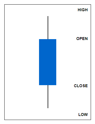
- 开盘价是当天股市开盘时的第一个交易价格。
- Close is the last traded price when the stock market ends for the day.
收盘价是当天股市收盘时的最后交易价格。 - High is the highest price traded during the day.
High 是当天交易的最高价格。 - Low is the lowest price traded during the day.
Low 是当天交易的最低价格。
Volume indicates the number of shares investors transacted that day.
交易量表示投资者当天交易的股票数量。
You can use the adv20 data field to access the 20-day average volume. If you want to calculate the average for a different number of days, you can use ts_mean(volume,N).
您可以使用 adv20 数据字段访问 20 天的平均交易量。如果要计算不同天数的平均值,可以使用 ts_mean(volume,N)。
📋 VWAP (成交量加权平均价格)
Additionally, VWAP can represent a day's stock price, which is the volume-weighted average price. Since low-volume trades might give a false picture of other price indicators like closing price, VWAP can be a better measure of that day's price. Let's look at this table:
此外,VWAP 可以代表一天的股票价格,即成交量加权平均价格。由于小批量交易可能会错误地反映其他价格指标(如收盘价),因此 VWAP 可以更好地衡量当天的价格。让我们看看这个表格:
Here, the VWAP is 11, resulting from dividing the sum of price times volume by the total volume sum. In formula terms, it's sum(price*volume)/sum(volume).
这里,VWAP 是 11,由价格乘以交易量之和除以总交易量总和得出。用公式来说,它是 sum(price*volume)/sum(volume)。
- perform well, while stocks that have performed poorly will continue to do so.
动量 - 假设过去表现良好的股票将继续表现良好,而表现不佳的股票将继续表现良好。- Momentum effect typically appears over longer periods (several months or more).
动量效应通常出现在较长时间(几个月或更长时间)内。
- Momentum effect typically appears over longer periods (several months or more).
- Reversion -The hypothesis is that if something increases today, it will fall tomorrow. And if something decreases today, it will increase tomorrow. This something can be anything: price, volume, correlation between two things or the other indicators/variables that you can think of while developing your alpha.
回归 - 假设是如果某物今天增加,明天就会下降。如果某件事今天减少,明天就会增加。这可以是任何东西:价格、交易量、两件事之间的相关性或您在开发 alpha 时可以想到的其他指标/变量。- Reversion effect appears over shorter periods (days or weeks).
回归效应在较短的时间段(几天或几周)内显示。
- Reversion effect appears over shorter periods (days or weeks).
我们应该尝试使用 VWAPP 实现一个回归 Alpha 吗?VWAP 是当天按交易量加权的平均价格,而收盘价是最后交易价格。通过比较 VWAP 和收盘价,我们可以了解最后交易价格与当天平均值的比较情况。例如,如果收盘价远高于 VWAP,我们可以解释为价格在收盘附近上涨。反之亦然。
Since reversion theory assumes prices return to their mean, we can implement an Alpha using the formula "vwap/close". This takes long positions when closing prices fall below VWAP, and short positions when they rise above it.
由于回归理论假设价格回到其均值,因此我们可以使用公式 “vwap/close” 实现 Alpha。当收盘价低于 VWAP 时,它需要多头头寸,当收盘价高于 VWAP 时,它需要多头头寸。
When you simulate this, you'll notice that while the Sharpe ratio is high, the turnover is excessive. According to submission criteria, turnover should be below 70% for submission. You can adjust turnover by applying operators (ex. trade_when) or changing settings (ex. Decay).
当您模拟此情况时,您会注意到,虽然夏普比率很高,但周转率过高。根据提交标准,提交的营业额应低于 70%。您可以通过应用运算符(例如 trade_when)或更改设置(例如 Decay)来调整周转率。
技术分析是一种分析方法,旨在根据历史价格和交易量数据预测未来价格走势。它基于市场参与者的心理和行为模式重复的假设,使用各种指标,例如图表模式、价格趋势、动量指标和移动平均线。以下是您可以在 Alpha 探索中使用的一些代表性指标:
- RSI (Relative Strength Index): A momentum indicator showing the degree of price increase/decrease
RSI (相对强弱指数): 显示价格上涨/下跌程度的动量指标 - Bollinger Bands: Sets upper/lower bands using standard deviation around a moving average
Bollinger Bands(布林带): 使用移动平均线周围的标准差设置上限/下限 - MACD (Moving Average Convergence Divergence): A trend indicator using the difference between short-term and long-term moving averages
MACD (Moving Average Convergence Divergence) (移动平均收敛散度): 使用短期和长期移动平均线之间差值的趋势指标
CLV = ((Close - Low) - (High - Close)) / (High - Low)
CLV = ((收盘价 - 最低价) - (最高价 - 收盘价)) / (最高价 - 最低价)
The CLV value ranges from 1 to -1, with these characteristics:
CLV 值的范围从 1 到 -1,具有以下特征:
- CLV close to 1 means closing price is near the high
CLV 接近 1 表示收盘价接近高点 - CLV close to -1 means closing price is near the low
CLV 接近 -1 意味着收盘价接近低点
CLV 是一个捕捉一天(短期)价格变化的指标。因此,它可能更适合在 PV Alpha 的两个主要分支(动量和反转)之间创建回归 Alpha。因此,以下想法可能是有效的:
When CLV is low (close to -1) → Buy position
当 CLV 较低(接近 -1)时→买入头寸
When CLV is high (close to 1) → Sell position
当 CLV 较高(接近 1)时 → 卖出头寸
提示: CLV 表达式的范围是 -1 到 1。
Write an alpha that allocates more positions to stocks with higher volume.
编写一个 alpha,将更多头寸分配给交易量更高的股票。
DECAY 4
 clv = ((close-low)-(high-close))/(high-low);
 -clv * rank(volume)
答:
DECAY 4
 clv = ((close-low)-(high-close))/(high-low);
 -clv * rank(volume)
使用所有四个数据字段创建夏普比率高于 1.4 的 Alpha: 最高价、最低价、收盘价、成交量 。
Momentum effect manifests differently depending on the time perspective:
动量效应根据时间视角的不同而表现不同:
- Short-term (less than 1 month): Reversion effect is stronger
短期 (不到 1 个月):回归效应更强 - Medium-term (quarter to year): Traditional momentum effect is most pronounced
中期 (季度至年):传统动量效应最为明显 - Long-term (over 12 months): Effect tends to gradually weaken
长期 (超过 12 个月):效果趋于逐渐减弱
The momentum effect can be implemented in various ways. The simplest method is calculating recent price increases. Shall we calculate an asset's price increase over one year? Since BRAIN only considers business days, a year's length is typically represented as 250 days (the number of business days in a year). We can measure the change in x over a year using the time series operator ts_delta(close,250)/ts_delay(close,250).
动量效应可以通过多种方式实现。最简单的方法是计算最近的价格上涨。我们应该计算资产一年内的价格上涨吗?由于 BRAIN 仅考虑工作日,因此一年的长度通常表示为 250 天(一年中的工作日数)。我们可以使用时间序列运算符 ts_delta(close,250)/ts_delay(close,250) 来衡量一年中 x 的变化。
但是,单独使用此公式不会产生良好的 Alpha 结果。一年期回报率受近期回报率的显著影响,包括短期回归效应。要在 BRAIN 中将动量效应实现为 Alpha,我们需要使用不同的方法或添加条件。
因此,为了更清楚地看到动量效应,我们可以使用以下方法:
- Apply delay to one-year returns to mitigate short-term reversion effects.
对一年期申报表应用延迟,以减轻短期回归效应。- ts_delay(ts_delta(close,250)/ts_delay(close,250),10)
ts_delay(ts_delta(收盘,250)/ts_delay(收盘,250),10)
- ts_delay(ts_delta(close,250)/ts_delay(close,250),10)
- Count the number of days with price increases over one year.
计算一年内价格上涨的天数。- ts_sum(returns>0? 1:0, 250) *
ts_sum(返回>0? 1:0, 250) *
- ts_sum(returns>0? 1:0, 250) *
* <condition>? <if_true>:<if_false> returns if_true value when the condition is true, and if_false value when it's not. if_else(<condition>,<if_true>,<if_false>) means the same thing.
* <condition>? <if_true>:<if_false> 在条件为 true 时返回 if_true 值,在条件不为 true 时返回 if_false 值。if_else(<condition>,<if_true>,<if_false>) 表示相同的内容。
ts_sum(if_else(greater(returns,0),1,0),250)
解析 ts_sum(if_else(greater(returns,0),1,0),250)
这个表达式是金融时间序列分析中的一个复合函数,用于统计过去 250 天内收益率为正的天数。下面我来逐步拆解它的逻辑:
函数拆解与执行流程
1. 内层函数 greater(returns,0)
- 功能:判断每日收益率是否大于 0。
- 输入:
returns是每日收益率序列。 - 输出:布尔值序列,收益率 > 0 时为
True,否则为False。
2. 中间函数 if_else(...)
- 功能:根据布尔值进行条件赋值。
- 逻辑:
plaintext
if returns[i] > 0:赋值为 1 else:赋值为 0 - 输出:由
1和0组成的序列,其中1代表当天收益率为正。
3. 外层函数 ts_sum(...,250)
- 功能:计算过去 250 天内的累积和。
- 滑动窗口:对每个时间点
t,统计[t-249, t]区间内所有1的总和。 - 输出:每个时间点对应的过去 250 天内正收益天数。
数学表达
对于时间序列 returns = [r₁, r₂, ..., rₜ],该函数计算:
plaintext
result[t] = ∑_{i=t-249}^{t} I(r_i > 0)
其中 I(r_i > 0) 是指示函数,当 r_i > 0 时为 1,否则为 0。
Python 实现示例
python
运行
import numpy as npdef ts_sum(if_else_result, window=250):"""计算滑动窗口内的累积和"""return np.convolve(if_else_result, np.ones(window), mode='valid')def greater(returns, threshold):"""判断序列中每个元素是否大于阈值"""return returns > thresholddef if_else(condition, value_if_true, value_if_false):"""根据条件进行赋值"""return np.where(condition, value_if_true, value_if_false)# 示例数据:生成1000天的随机收益率
np.random.seed(42)
returns = np.random.normal(0.0005, 0.01, 1000)  # 假设日均值0.05%,标准差1%# 计算正收益天数
condition = greater(returns, 0)
binary_result = if_else(condition, 1, 0)
positive_days = ts_sum(binary_result, window=250)# 输出前10个结果
print("过去250天内正收益天数:", positive_days[:10])
实际应用场景
-
市场强度指标:
- 正收益天数占比高(如超过 130 天),表明市场处于强势。
-
胜率分析:
- 对策略回测而言,该指标反映策略在历史上的胜率。
-
风险评估:
- 连续低正收益天数可能预示市场风险上升。
注意事项
-
边界处理:
- 对于前 249 天的数据,无法形成完整窗口,需特殊处理(如返回 NaN 或 0)。
-
参数选择:
window=250通常对应一年交易日,但需根据实际需求调整。
-
与其他指标结合:
- 单独使用意义有限,建议结合收益率均值、波动率等指标综合分析。
这个函数本质是一个动量类指标,通过统计正收益天数的频率来衡量市场或资产的强势程度。
编辑
分享
如何解释ts_sum(if_else(greater(returns,0),1,0),250)的输出结果?
ts_sum(if_else(greater(returns,0),1,0),250)和ts_sum(if_else(greater(returns,0),1,0),120)有什么区别?
ts_sum(if_else(greater(returns,0),1,0),250)的计算结果可以用于哪些分析场景?
解析 ts_sum(if_else(greater(returns,0),1,0),250)
这个表达式是金融时间序列分析中的一个复合函数,用于统计过去 250 天内收益率为正的天数。下面我来逐步拆解它的逻辑:
函数拆解与执行流程
1. 内层函数 greater(returns,0)
- 功能:判断每日收益率是否大于 0。
- 输入:
returns是每日收益率序列。 - 输出:布尔值序列,收益率 > 0 时为
True,否则为False。
2. 中间函数 if_else(...)
- 功能:根据布尔值进行条件赋值。
- 逻辑:
plaintext
if returns[i] > 0:赋值为 1 else:赋值为 0 - 输出:由
1和0组成的序列,其中1代表当天收益率为正。
3. 外层函数 ts_sum(...,250)
- 功能:计算过去 250 天内的累积和。
- 滑动窗口:对每个时间点
t,统计[t-249, t]区间内所有1的总和。 - 输出:每个时间点对应的过去 250 天内正收益天数。
数学表达
对于时间序列 returns = [r₁, r₂, ..., rₜ],该函数计算:
plaintext
result[t] = ∑_{i=t-249}^{t} I(r_i > 0)
其中 I(r_i > 0) 是指示函数,当 r_i > 0 时为 1,否则为 0。
Python 实现示例
python
运行
import numpy as npdef ts_sum(if_else_result, window=250):"""计算滑动窗口内的累积和"""return np.convolve(if_else_result, np.ones(window), mode='valid')def greater(returns, threshold):"""判断序列中每个元素是否大于阈值"""return returns > thresholddef if_else(condition, value_if_true, value_if_false):"""根据条件进行赋值"""return np.where(condition, value_if_true, value_if_false)# 示例数据:生成1000天的随机收益率
np.random.seed(42)
returns = np.random.normal(0.0005, 0.01, 1000)  # 假设日均值0.05%,标准差1%# 计算正收益天数
condition = greater(returns, 0)
binary_result = if_else(condition, 1, 0)
positive_days = ts_sum(binary_result, window=250)# 输出前10个结果
print("过去250天内正收益天数:", positive_days[:10])
实际应用场景
-
市场强度指标:
- 正收益天数占比高(如超过 130 天),表明市场处于强势。
-
胜率分析:
- 对策略回测而言,该指标反映策略在历史上的胜率。
-
风险评估:
- 连续低正收益天数可能预示市场风险上升。
注意事项
-
边界处理:
- 对于前 249 天的数据,无法形成完整窗口,需特殊处理(如返回 NaN 或 0)。
-
参数选择:
window=250通常对应一年交易日,但需根据实际需求调整。
-
与其他指标结合:
- 单独使用意义有限,建议结合收益率均值、波动率等指标综合分析。
这个函数本质是一个动量类指标,通过统计正收益天数的频率来衡量市场或资产的强势程度。
When creating Alpha, you can fine-tune Alpha positions using conditions, using operators like if_else() or trade_when().
创建 Alpha 时,您可以使用条件微调 Alpha 位置,使用 if_else() 或 trade_when() 等运算符。
您可以使用常用逻辑运算符(>、<、>=、<=、== 等)创建条件。例如,如果您只想在交易量高于平时(20 天平均值)时更改位置,则可以将条件设置为交易量 > adv20。以下是一些需要考虑的条件,但您可以创建所需的任何条件。请注意,设置过于严格的条件可能会减少数据点的数量并增加过度拟合的风险。
在实现 Alpha 时,有时您需要根据特定条件返回不同的值。if_else 运算符是一个基本但功能强大的运算符,可让您简单地实现条件逻辑。
You can also use if_else in the form of condition? if_true:if_false. For example, ts_sum(returns>0? 1:0, 250) uses this format.
你也可以用 condition if_else 的形式 if_true:if_false。 例如,ts_sum(returns>0? 1:0, 250) 使用此格式。
使用 trade_when 运算符,您可以决定何时更改 Alpha 中的值。trade_when 运算符仅在特定条件下更改 Alpha 值,否则保持较早的位置。
trade_when takes three inputs: entry condition, Alpha expression, and exit condition.
trade_when 接受三个输入: 进入条件、Alpha 表达式和退出条件 。
- When the entry condition is true, it updates the Alpha expression value daily.
当输入条件为 true 时,它每天更新 Alpha 表达式值 。 - When the exit condition is true, it liquidates the position (NaN).
当退出条件为 true 时, 它会清算仓位 (NaN)。 - When both are false, it maintains the last Alpha value from when the entry condition was true.
当两者都为 false 时,它将保持进入条件为 true 时的最后一个 Alpha 值 。让我们设置入场条件。基于动量在成交量激增时起作用的假设,我们可以使用以下方法检测成交量增加:
- volume > adv20 #adv20: 20-day average volume
交易量 > adv20 #adv20:20 天平均交易量 - volume > ts_mean(volume, N_DAYS)
Volume > ts_mean(volume, N_DAYS) - volume * vwap > ts_mean(volume * vwap, N_DAYS)
交易量 * VWAP > ts_mean(交易量 * VWAP, N_DAYS) -
You can test different values for N_DAYS.
您可以测试 N_DAYS 的不同值。Since momentum is a long-term effect, it's effective to set the exit condition to –1 to keep positions longer once established. Or you can set your own exit condition which you think is effective.
由于动量是一种长期影响,因此将退出条件设置为 –1 以在建立后保持更长时间是有效的。或者您可以设置您认为有效的退出条件。
Also, since momentum effects tend to occur across industries rather than within them, it's better to set Neutralization options to avoid overly detailed grouping such as Market or Sector.
此外,由于动量效应往往发生在行业之间,而不是行业内部,因此最好设置 Neutralization 选项以避免过于详细的分组 ,例如 Market 或 Sector。
你提供的代码是一个量化交易策略,结合了两个关键信号:正收益天数频率和成交量异常。下面我来详细拆解这个策略的逻辑和应用场景。
- 功能:统计过去 250 个交易日中,收益率为正的天数总和。
- 信号含义:
positive_days越大,说明近期市场强势(上涨天数多)。- 典型阈值:若
positive_days > 130,意味着超过半数时间市场上涨。
)


Java/python/JavaScript/C/C++/GO最佳实现)


![[特殊字符] UI-Trans:字节跳动发布的多模态 UI 转换大模型工具,重塑界面智能化未来](http://pic.xiahunao.cn/[特殊字符] UI-Trans:字节跳动发布的多模态 UI 转换大模型工具,重塑界面智能化未来)


)
